9
Joel Bruneau and Clinton Mahoney
Learning Objectives
- Explain how competitive, price-taking firms decide on output levels
- Describe how competitive firms make decisions on short-run output and whether to shut down if they experience negative profit
- Describe competitive firms’ long-run supply curves and how firm entry and exit affects the long-run market equilibrium
- Demonstrate how increasing and decreasing cost industries affect the long run market supply curve
Module 10: Profit Maximization and Supply
The Policy Question: Will a Carbon Tax Harm the Economy?
Carbon emissions into the atmosphere have been identified as the key component in global warming due to human activity. We know from earlier modules that the cost of consumption influences human choices. Therefore a very popular policy proposal to address global warming is to impose a tax on carbon at the source. For example, the state of California and the Canadian province of British Columbia began imposing a carbon tax in 2015 and 2008, respectively. Carbon taxes generally increase the price of fossil fuels, which have a large carbon component. The result is an increase in energy prices for all users. Critics of these policies suggest that carbon taxes would have an adverse impact on the economy greater than any potential benefit.
To analyze the impact on the economy, we must start with the individual actors upon which the economy depends: the firms themselves. This module examines how firms make decisions about how much to produce and how their profits are determined. Once we have developed a general model, we can use it to analyze the impact of a carbon tax on individual firms, understand the firm-level implications of the tax, and know the right questions to ask when trying to determine the cost and benefits of a carbon tax.
In this module we will study the supply side of markets: how firms’ cost conditions define and affect their supply curves and the market supply curve. By summing up all producers’ supply curves within a given industry, we can construct a market supply curve just as we constructed the market demand curve from individual demand curves. When we have both market demand and market supply we will be able to study market equilibrium in Section 3.
Exploring the Policy Question
How does a tax on carbon affect individual firms’ output and profits?
10.1 Output Decisions for Price–Taking Firms
Learning Objective 10.1: Explain how competitive, price-taking firms decide on output levels.
10.2 Short-Run Supply
Learning Objective 10.2: Describe how competitive firms make decisions on short-run output and whether to shut down if they experience negative profit.
10.3 Long-Run Supply and Market Equilibrium
Learning Objective 10.3: Describe competitive firms’ long-run supply curves and how firm entry and exit affects the long-run market equilibrium.
10.4 Heterogeneous Firms and Constant, Increasing and Decreasing Cost Industries
Learning Objective 10.4: Demonstrate how increasing and decreasing cost industries affect the long run market supply curve.
10.1 Output Decisions for Price Taking Firms
LO 10.1: Explain how competitive, price-taking firms decide on output levels.
Before considering the production decisions of firms, we need to understand a few foundation ideas. First, we are focusing on the behavior of price-taking firms. A firm is said to be a price taker when it has no ability to influence the price the market will pay for its product; it must take the market price as determined by the laws of supply and demand in a competitive market. A perfectly competitive market is a market in which there are many firms so that each individual firm’s output has no impact on market equilibrium, output is identical across firms, firms have the same access to inputs and technology and consumers have perfect information about prices. All firms in a perfectly competitive market are price takers.
Second, we are focusing on firms that are motivated by profit. Many publicly- and privately-owned firms have one main objective: to maximize profits. Not-for-profit firms seek to maximize some other objective, like providing a social service such as mental health care to the greatest number of people in need, but these are a tiny fraction of all firms in the world. In this module we will assume that firms’ objectives are to maximize profits.
A firm’s profit (π) is the difference between its total revenue and its total cost:
The total revenue is the quantity of the goods produced multiplied by the sales price of those goods.
The total cost is the total cost curve C(Q) introduced in Module 7 and represents the economic cost. The economic cost is the cost inclusive of all opportunity costs, so it includes both explicit costs and implicit costs. This is distinct from the accounting cost which includes only the explicit costs, or those you would see in an accounting spreadsheet of the firm’s costs. So equation (9.1) is an expression of the economic profits of the firm, which consider economic costs. In economics, we focus exclusively on economic profits, because this is the relevant measure when it comes to decision-making.
To understand the difference between accounting cost and economic cost, imagine deciding whether to open up and run a small business making and selling soap infused with organic botanicals. Suppose you figure that your business will achieve annual sales of $230,000 and your out-of-pocket costs for the ingredients, equipment rental, property rental, etc., is $155,000 annually. Your accounting profits after a year would be $230,000-$155,000= $75,000, a pretty decent return.
But should you go ahead and start the business? To answer that you need to think about your opportunity cost. What would you do instead if you decided not to start your own business? Imagine that your friend has offered to hire you to work in her firm and she will pay you an annual salary of $90,000. Imagine also that you think you would be equally satisfied working with your friend as running your own business. With this in mind, your annual economic costs of running your business is $155,000 + $90,000 = $245,000. So your annual economic profit would be $230,000 – $245,000 = -$15,000. The answer is now clear–your best decision is to not run a business making soap but to work with your friend.
Let’s now turn to the output choice of a profit maximizing, price-taking firm. The objective of maximizing profit means that firms must choose the output level that maximizes the difference between total revenue and total profit. To determine this specific level of output the firm must ask how the production of one more unit of output contributes to both the total revenue and the total cost. For example, if a car manufacturer can produce one more car at a marginal cost of $15,500 and sell that car for a marginal revenue of $17,000, it knows that by producing the extra car its profits will increase by $1,500. Note that this is not the same as knowing that profits are positive because the calculation does not include fixed costs. Similarly if the additional car has a marginal cost of $18,000 to produce and can be sold for $17,000 then the manufacture and sale of this car would reduce profits by $1,000.
The term marginal revenue (MR), used in our example above, refers to the change in total revenue from a one-unit change in quantity produced. Marginal revenue is expressed
[latex]MR=\Delta TR/\Delta Q[/latex]
For a price-taking firm this increase in revenue from the sale of an additional unit is exactly the price of that unit. In other words, for a price-taking firm MR=P.
CALCULUS APPENDIX:
The marginal revenue is the rate of change of total revenue as output increases, or the slope of the total revenue function, TR(Q). To find this we take the derivative of the total revenue function: [latex]MR(Q)=\frac{dTR(Q)}{dQ}[/latex]
Any profit-maximizing firm would like to continue to increase output as long as marginal revenue is larger than marginal cost. A profit-maximizing firm would also like to reduce output as long as marginal revenue is lower than marginal cost. The incentive to increase or decrease output stops exactly when marginal revenue equals marginal cost. This is known as the profit maximization rule: profit is maximized when output is set where marginal revenue equals marginal cost.
From Module 9 we learned that marginal cost (MC) is the additional cost incurred from the production of one more unit of output: MC=∆C/∆Q. Since the profit maximizing rule stipulates that output should be set where marginal revenue equals marginal cost and since marginal revenue for a price-taking firm is the price of the good, we know that at the profit maximizing output level for the firm, P=MC(Q).
The expression P=MC(Q) gives us a relationship between the price, P, of a good and the quantity, Q, that a profit-maximizing, price-taking firm will produce at that price. In other words, it gives us the individual firm’s supply curve. Figure 10.1.1 illustrates this relationship.
Figure 10.1.1 Profit Maximization for a Price-Taking Competitive Firm
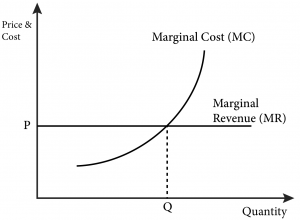
In Figure 10.1.1 we see that the firm’s profit maximizing level of output is where marginal revenue equals marginal cost. For a price-taking firm, marginal revenue is equal to the price. So, as price increases the firm will increase production and when the price decreases the firm will decrease production.
10.2 Short-Run Supply
LO 10.2: Describe how competitive firms make decisions about short-run output and whether to shut down if they experience negative profit.
To understand the short-run supply decision of the firm we have to be able to measure the firm’s profits. The profit maximization rule, to set output such that marginal revenue equals marginal cost ensures that the firm is maximizing profit, but it does not ensure that the firm is making positive profits. In other words, following the MR=MC rule means that the firm is doing the best it can, which could be minimizing losses instead of making positive profits.
To see how we go from the output decision to profits consider the following:
[latex]\Pi=TR-TC[/latex]
[latex]TR=P x Q[/latex]
[latex]TC=ATC xQ\,(since\,ATC=\frac{TC}{Q})[/latex]
Thus,
[latex]\Pi=(PxQ)-(ATCxQ)[/latex]
[latex]=(P-ATC)xQ[/latex]
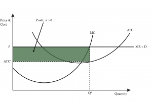
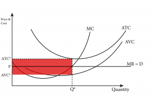
Since Q*, the quantity for which MR=MC, is always positive or zero, whether profit (π) is positive or negative depends on the price (P) relative to the average total cost at that particular Q* (ATC*). If P>ATC* then π > 0 as seen in Figure 10.2.1. In the figure, profits (π) are represented graphically by the shaded area. Notice that the height of the rectangular shaded area is P-ATC, and the width is Q. Since the area of a rectangle is height times width, the area of this rectangle equals the profit.
Figure 10.2.1 Positive Profit: P > ATC*
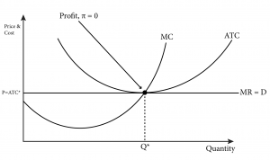
If P=ATC*, then π=0, as seen in Figure 10.2.2
Figure 10.2.2 Zero Profit: P = ATC*
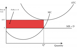
If P<ATC*, then π<0, as seen in Figure 10.2.3
Figure 10.2.3 Negative Profit (Loss): P < ATC*
It is tempting to think that if profit is negative, the firm should immediately shut-down or cease production of the good. But remember that in the short run, there are fixed inputs that cannot be adjusted immediately. For example, suppose the soap selling business requires the leasing of a storefront. This lease is a three-month lease and the three monthly payments of $1000 each must be made regardless of whether the store is open or closed. Now suppose that the business is making enough revenue to cover all of the variable costs like the ingredients for the soap, the electricity bill, your own salary and part of the lease, perhaps $500 of the $1000. If you continue to operate the store, you will lose $500 per month – the part of the lease payment not covered by revenues. If you shut down you will loose $1000 per month until the lease runs out because although there are no variable costs there also is no revenue.
Consider the following expression for profit:
π=TR-TC
=TR-FC+VC
=TR(Q)-FC-VC(Q)
The third line in this expression shows that TR and VC are both functions of Q, so if Q=0, then TR=0 and VC=0 as well. Shutting down means to set Q=0 so,
Level of profit if the firm shuts down: π=0-FC-0=-FC
So in the short-run a firm should only shut down if the total revenue is lower than the variable cost, which is the same as the price being lower than the average variable cost.
Figure 10.2.4 illustrates the situation where the firm is generating a negative profit but should continue to operate in the short run. At Q* the firm is making negative economic profits because (P-ATC*) is negative (π=(P-ATC*)Q*). However, the firm is covering all of its variable costs (P>AVC*) and part of its fixed costs. Of course, when the short run ends because the firm is able to adjust its previously fixed input, the firm should shut down if its total revenue is still lower than total cost.
Figure 10.2.4: Negative Profit but in the Short-Run Firm Should Continue to Operate
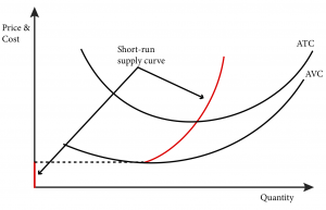
This understanding of the short-run output decision allows us to derive the firm’s short-run supply curve. As long as the market price is above the firm’s average variable cost, the firm will choose to produce output where P=MC. In other words, the firm’s marginal cost curve above the AVC curve is the firm’s supply curve. When price is below AVC the firm chooses not to produce any output at all so the supply for prices below AVC is zero. Figure 10.2.5 illustrates the firm’s short run supply curve.
Figure 10.2.5: Competitive Firm’s Short-Run Supply Curve
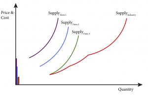
Every firm in a given industry has a short-run supply curve, but its precise shape depends on the firm’s cost structure – the shape and location of its MC and AVC curves. Because each individual firm supplies a certain amount of output at every price, we can derive the industry supply curve by simply adding up these outputs across all firms in the industry. When we do this, we must take care to sum the quantities at every price, not the other way around.
Figure 10.2.6 shows how summing up all individual short-run supply curves yields the industry short-run supply curve, which represents the quantity supplied in the short run at every price.
Figure 10.2.6 Deriving an Industry Short-Run Supply Curve
10.3 Long-Run Supply and Market Equilibrium
LO 10.3: Describe a competitive firm’s long-run supply curves and how firm entry and exit affects the long-run market equilibrium.
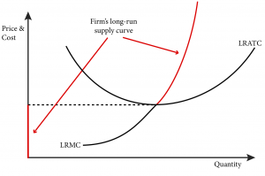
In the long run, firms do not have any fixed costs; all production costs are variable. So a firm’s profitability is determined solely by the long-run average total cost curve. A profit maximizing firm still sets output such that marginal revenue equals marginal cost, and since marginal revenue for a perfectly competitive firm is equal to the market price, the marginal cost curve above the long-run average total cost curve (LRATC) represents the firm’s supply curve.
As in the short-run case, the firm’s profits depend on the price relative to the long-run average total cost at the optimal output level for the firm, Q*. In Figure 10.3.1, the price is above LRATC so the firm is making positive profits. As long as profits are not negative the firm will continue to produce. So the portion of the long-run marginal cost (LRMC) that lies above the LRATC is the firm’s supply curve as seen in Figure 10.3.2:
Figure 10.3.1: Positive Profits in the Long Run
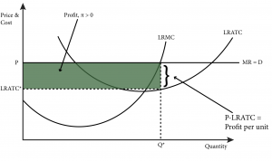
Figure 10.3.2: The Long–Run Supply Curve of a Perfectly Competitive Firm
To derive the long-run market supply curve, we have to think about how firms enter and exit industries in the long run. We assume perfectly competitive industries have free entry and free exit: there are no special costs, such as technical or legal barriers, to firms entering and exiting the industry. This assumption is critical to perfect competition. Barriers that block firms from entering or exiting will create an environment that has only limited competition.
Barriers to Free Entry and Free Exit
Barriers to entry and exit can be legal, such as patents that limit the production of a good to the firm that invented it, or technical, such as the cost of setting up a network of wires to homes for a company that wishes to provide cable television services. We will study such barriers in more detail in Module 16 when we study monopolies.
If free entry and exit exist, the next question to answer is when will firms choose to enter and exit a market? To answer this question, we will assume for now that all firms in a market are homogeneous. That is, they have identical technologies and cost structures, or more simply they all have the same LRATC and LRMC curves. We will examine firms that have different costs in the next section of this module.
Figure 10.3.1 illustrates the case where the market price is such that the firm is making positive profits. Positive profits in this case mean that the firm is getting better than normal returns, or that this is an exceptionally profitable market to be in. Other firms, not currently in the market, will see these profits and decide that this is a good market to enter. When new firms enter the market they provide their output to the total supply and the market supply increases.
Figure 10.3.3: New Entrants Increase Market Supply and Lower Equilibrium Price

As illustrated in Figure 10.3.3, as new firms, drawn by positive profits, enter the market, the added supply lowers the equilibrium price—the price at which quantity demanded equals the quantity supplied. This lowering of the equilibrium price lowers all firms’ profits. Entry will continue to occur as long as firms’ profits are positive, and so this process will continue until the equilibrium price has reached the point where the LRATC and the LRMC cross, or where there are zero profits as shown in Figure 10.3.4
Figure 10.3.4: Equilibrium With Zero Profits
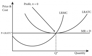
Equilibrium with zero profits actually includes two kinds of equilibrium:
- a market equilibrium where the price equates the quantity supplied to the quantity demanded;
- an equilibrium in the number of firms in the market as the zero profit experienced by the existing firms in the market does not attract any new entrants.
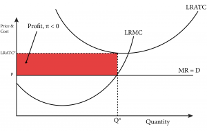
The market exit dynamics work similarly to the market entry dynamics. Firms that are currently producing and supplying their output to a market where the equilibrium price is below their LRATC are making negative profits, which by the definition of opportunity cost means that other opportunities exist that yield higher returns. This fact will cause existing firm to want to exit the market.
A firm’s profit is negative when the equilibrium price is below the firm’s LRATC at its profit maximizing level of output. In this case, profit maximization is synonymous with loss minimization – the firm is making the best output choice it can. Figure 10.3.5 illustrates a situation of long-run negative profits for a firm.
Figure 10.3.5: Negative Profits in the Long Run
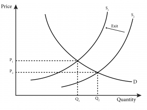
Will all firms exit the market when profits are negative? No, because as the first firms exit the market, supply will fall and the equilibrium price will rise. Figure 10.3.5 illustrates this behavior graphically. Once the price rises to the point where it equals LRATC there will no longer be an incentive for firms to leave the market.
Figure 10.3.6: Exiting Firms Cause Market Supply to Decrease and a Rise in the Equilibrium Price
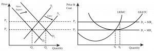
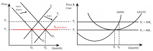
The long-run entry and exit dynamic allows us to understand the long-run market supply curve. Entry and exit dynamics will always force the price back to P1 in the long-run as new firms enter to satisfy any new demand and existing firms exit when demand falls. The resulting long-run supply curve is horizontal, as shown in Figure 10.3.7.
Figure 10.3.7: The Long-Run Market Supply Curve
10.4 Heterogeneous Firms and Increasing and Decreasing Cost Industries
LO 10.4: Show how increasing and decreasing cost industries affect the long-run market supply curve.
In the previous section we explicitly assumed homogeneous firms—that is, firms all having identical costs. We also assumed, implicitly, that costs were constant as industry output changed. In this section we will study what happens when these assumptions do not hold.
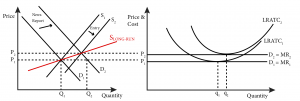
Consider first a number of firms that all produce the same good but which all have different costs—that is, heterogeneous firms. It makes sense that the firms with the lowest costs would be the first to provide their output to the market and that they would experience positive profit. Their success would attract new entrants to the market, just as in the case of homogeneous firms. Each new entrant can be expected to be the next-lowest cost firm. Entry will continue until profits reach zero for the most recent entrant, causing it to become the last entrant.
Zero profits will happen when the supply increases enough to push price down to equal the marginal cost of the very last entrant. Since the entrants that came before the last one all have lower costs, they will all continue to experience positive profits. No other firms will enter after the last, zero-profit entrant because they are, by assumption, higher cost firms and will earn negative profits if they do so. After profits reach zero, new entrants will be drawn in only if the price rises.
In the case of heterogeneous firms, the long-run supply curve will be upward sloping even in the case of perfect competition, as seen in Figure 10.4.1
Figure 10.4.1: Long-Run Supply in the Case of Firms With Different Costs
The second assumption that was implicit in the previous section is that firms are in a constant-cost industry: industries where firms’ costs do not change as industry output changes. So, no matter how much total output there is in the industry, all the LRATC curves remain in the same place.
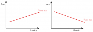
This assumption does not hold for many industries. Some industries are increasing-cost industries: industries where firms’ costs increase as industry output increases. This can happen because as an industry expands the demand for inputs or industry-specific capital increases, which can cause the prices to rise. For example, if the demand for coffee increases due to positive news about the health benefits of consumption, the demand for coffee beans will increase as well, which could lead to an increase in their price. As the industry output increases, the costs of all firms will increase and the long-run supply curve will slope upward, as shown in Figure 10.4.2(a).
Other industries might be decreasing-cost industries: industries where firms’ costs decrease as industry output increases. This could be because these industries have increasing returns to scale, or because increased demand for inputs and capital leads to increased returns to scale on the part of the firms that supply these goods. For example, if the demand for coffee increases the demand for espresso machines, espresso machine manufacturers might invest in cost saving technologies such as automating parts of the assembly process. As the coffee industry output increases, the cost of espresso machines decreases, the costs of coffee shops decrease, and the long-run supply curve would be downward sloping, as shown in Figure 10.4.2(b).
Figure 10.4.2: Long-Run Supply Curves for Increasing and Decreasing Cost Industries
The heterogeneity of firm’s cost structures, and the fact that many or most industries could be described as increasing cost industries, lead economists to generally draw the market supply curve as upward sloping. From the information learned in this module you can now see where that market supply curve comes from – the firms themselves.
SUMMARY
Review: Topics and Related Learning Outcomes
10.1 Output Decisions for Price–Taking Firms
Learning Objective 10.1: Explain how competitive, price-taking firms decide on output levels.
10.2 Short-Run Supply
Learning Objective 10.2: Describe how competitive firms make decisions on short-run output and whether to shut down if they experience negative profit.
10.3 Long-Run Supply and Market Equilibrium
Learning Objective 10.3: Describe competitive firms’ long-run supply curves and how firm entry and exit affects the long-run market equilibrium.
10.4 Heterogeneous Firms and Constant, Increasing and Decreasing Cost
Industries
Learning Objective 10.4: Demonstrate how increasing and decreasing cost industries affect the long run market supply curve.
Learn: Key Terms and Graphs
Terms
Graphs
Profit Maximization for a Price-Taking Competitive Firm
Negative Profit but in the Short-Run Firm Should Continue to Operate
Competitive Firm’s Short-Run Supply Curve
Positive Profits in the Long-Run
The Long Run Supply Curve of a Perfectly Competitive Firm
New Entrants Increase Market Supply and Lower Equilibrium Price
Negative Profits in the Long-Run
Exiting Firms Cause Market Supply to Decrease and a Rise in the Equilibrium Price
The Long-Run Market Supply Curve
Long-Run Supply in the Case of Firms With Different Costs
Long-Run Cost Curves for Increasing and Decreasing Cost Industries
Equations
Supplemental Resources
Practice Questions
YouTube Videos
These videos from the YouTube channel ‘Department of Economics’ may be helpful.
- Intermediate Microeconomics: Profit Maximization – YouTube
- Intermediate Microeconomics: Characterization of Profit Maximization – YouTube
- Intermediate Microeconomics: Profit Graphing Rules – YouTube
- Intermediate Microeconomics: Perfect Competition – YouTube
- Intermediate Microeconomics: Shutdown Rule – YouTube
- Intermediate Microeconomics: Short-Run Supply Curve (Type 2) – YouTube
- Intermediate Microeconomics: Short-Run Supply Curve Detail (Type 2) – YouTube
- Intermediate Microeconomics: Short-Run Simple Profit Graph (Type 2) – YouTube
- Intermediate Microeconomics: Short-Run Further Profit Graphs (Type 2) – YouTube
- Intermediate Microeconomics: Short-Run Profit Graph (Type 1) – YouTube
- Intermediate Microeconomics: Long-Run Competitive Pricing (Types A and B) – YouTube
- Intermediate Microeconomics: Long-Run Competitive Pricing (Types C and D) – YouTube
- Intermediate Microeconomics: Discontinuous Supply – YouTube
- Intermediate Microeconomics: Very Long Run – YouTube
- Intermediate Microeconomics: Equality of Marginal Products – YouTube
- Intermediate Microeconomics: Equality of MR’s & MC’s – YouTube
Policy Example
Policy Example: Will a Carbon Tax Harm the Economy?
Learning Objective: Predict the effect of a carbon tax on the supply and profit maximization decisions of firms on which it is imposed.
On July 1, 2008, in response to mounting evidence that human activity is contributing to global climate change and that carbon emissions are a key factor in rising earth temperatures; the Canadian province of British Columbia began collecting a tax on carbon emissions. In so doing, British Columbia became the first North American jurisdiction to levy a carbon tax.
The government of British Columbia charges a tax on revenue from the sale of all fuels: gasoline, diesel, natural gas, propane, jet fuel and coal. This taxis neutral, meaning the proceeds are returned to the citizens of the province through a reduction in income taxes and tax credits.
Though a carbon tax is a popular policy proposal for groups concerned about climate change and greenhouse gases, pro-business groups generally resist it, arguing that carbon taxes would do great harm to the economy. In this module we have studied how cost conditions translate into firm and market supply. Given this analysis we can come up with a prediction about the way that a carbon tax would affect firms’ production behavior.
Carbon taxes raise the price of energy, which is a production input. Energy usage generally, but not always, varies with the level of output. More intense production is generally associated with higher energy use. So we can assume that the energy input of firms is a variable cost. This means that an increase in the cost of energy will increase not only the total costs of the firms but their marginal costs as well. In Figure 1 we can see the resulting impact on firms and their marginal cost curves.
Figure 1: Effect of an Increase in Variable Cost
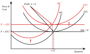
From this we can anticipate that firms’ supply curves will rise and that the new equilibrium price will increase. So business groups have a legitimate point in worrying about the effect of a carbon tax on firms’ costs. The effect on an individual firm is clear from Figure 1 – this tax will lead to it to charge higher prices and reduce output.
However, this is only part of the story. Revenue neutral carbon taxes will increase demand through income tax rebates and credits, which would serve to raise the equilibrium price. This could offset, at least in part the rise in costs. A true analysis of this policy would also include the economic impact of climate change itself and the benefit of carbon mitigation. This is a subject we will return to in Module 22: Externalities.
Exploring the Policy Question
- If a carbon tax is imposed, the costs in a perfectly competitive industry would likely rise. If firms make zero profits prior to the tax and zero profits after the tax, is it correct to say that there is no net effect of the tax?
- Another policy response to combat carbon emissions is to mandate reductions in energy usage on the part of firms. Using the theory of profit maximizing competitive firms, analyze the impact of this alternate policy.
- What else would you want to know about carbon emissions, climate change and the economy to give a full cost benefit analysis of a carbon tax?
Candela Citations
- Authored by: Joel Bruneau & Clinton Mahoney. License: CC BY-NC-SA: Attribution-NonCommercial-ShareAlike
- Module 9: Profit Maximization and Supply. Authored by: Patrick Emerson. Retrieved from: https://open.oregonstate.education/intermediatemicroeconomics/chapter/module-9/. License: CC BY-NC-SA: Attribution-NonCommercial-ShareAlike
- Profit Maximization. Authored by: Preston McAfee & Tracy R Lewis. Retrieved from: https://resources.saylor.org/wwwresources/archived/site/textbooks/Introduction%20to%20Economic%20Analysis.pdf. License: CC BY-NC-SA: Attribution-NonCommercial-ShareAlike
is a firm that has no ability to influence the price the market will pay for its product; it must take the market price as determined by the laws of supply and demand in a competitive market
a market in which there are many firms so that each individual firm’s output has no impact on market equilibrium, output is identical across firms, firms have the same access to inputs and technology and consumers have perfect information about price; all firms in a perfectly competitive market are price takers
is the difference between its total revenue and its total cost
is the cost inclusive of all opportunity costs, so it includes both explicit costs and implicit costs
includes only the explicit costs, or those you would see in an accounting spreadsheet of the firm’s costs
refers to the change in total revenue from a one-unit change in quantity produced
a rule that states that a firm should set output such that marginal revenue equals marginal cost to maximize profit in a competitive market
there are no special costs, such as technical or legal barriers, to firms entering the industry
there are no special costs, such as technical or legal barriers, to firms exiting the industry
the price at which quantity demanded equals the quantity supplied
industries where firms’ costs do not change as industry output changes; so, no matter how much total output there is in the industry, all the LRATC curves remain in the same place
industries where firms’ costs increase as industry output increases; this can happen because as an industry expands the demand for inputs or industry-specific capital increases, which can cause the prices to rise
industries where firms’ costs decrease as industry output increases; this could be because these industries have increasing returns to scale, or because increased demand for inputs and capital leads to increased returns to scale on the part of the firms that supply these goods
is the additional cost incurred from the production of one more unit of output

