
20
Joel Bruneau and Clinton Mahoney
Learning Objectives
- Explain the difference between partial and general equilibrium
- Draw an Edgeworth box for a trading economy and show how a competitive equilibrium is Pareto efficient
- Demonstrate how prices adjust to create a competitive equilibrium that is Pareto efficient form any initial allocation of goods
- Draw a production possibility frontier and explain how the mix of production is determined in equilibrium and how productive efficiency is guaranteed
Module 20: General Equilibrium
Policy Example: Should the Government Try to Address Growing Inequality Through Taxes and Transfers?
Rising income inequality in the United States has received a lot of attention in the last few years. As the graph below illustrates, since 1970, there has been a dramatic increase in the concentration of wealth at the top of the income distribution.
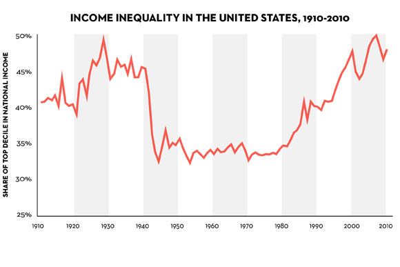
Recently, there has been a renewed emphasis on raising minimum wages as one way to try and address income inequality. But a more fundamental policy to address income inequality is a more aggressive tax and transfer policy where a larger share of the income of the top earners is collected in taxes and then redistributed to low income earners through tax credits. Critics of this policy worry about the effect such a policy will have on the economy arguing that it discourages investment and entrepreneurship and is inefficient.
Exploring the Policy Question
- Do tax and transfer schemes necessarily lead to inefficiency?
20.1 Partial Versus General Equilibrium
Learning Objective 20.1: Explain the difference between partial and general equilibrium.
20.2 Trading Economy: Edgeworth Box Analysis
Learning Objective 20.2: Draw an Edgeworth box for a trading economy and show how a competitive equilibrium is Pareto efficient.
20.3 Competitive Equilibrium: Edgeworth Box With Prices
Learning Objective 20.3: Demonstrate how prices adjust to create a competitive equilibrium that is Pareto efficient form any initial allocation of goods.
20.4 Production and General Equilibrium
Learning Objective 20.4: Draw a production possibility frontier and explain how the mix of production is determined in equilibrium and how productive efficiency is guaranteed.
20.1 Partial Versus General Equilibrium
Learning Objective 20.1: Explain the difference between partial and general equilibrium.
In all of our previous examinations of markets, we implicitly assumed that changes in other markets do not effect the market we are studying. Though we talked about complements and substitutes and cross-price elasticities we did not explicitly consider the interaction between markets. What we were doing is called a partial-equilibrium analysis: studying the changes in a single market in isolation. This is a useful technique in for it allows us to focus on one market and do comparative static analyses without having to try and figure out all of the interactions with other markets. The insight gained from this analysis is generally pretty accurate if a market does not have a lot of linkages. For example the market for biodiesel fuel – a type of diesel fuel produced from waste vegetable oils and animal fat – in the united states is extremely small and a spike in production costs that increases the price of biodiesel is unlikely to have much of an impact on other markets, even automobiles. Even if a market is likely to have large spillover effects on other markets, those effects could take a while to materialize so in the short-term partial equilibrium analyses might me reasonably accurate.
However, there are other markets in which the linkages are quite large. Take, for example, the market for crude oil. Crude oil prices affect retail gasoline prices, the market for automobiles and so on. In order to more accurately analyze these markets, in this module we will relax this assumption and explicitly study the interaction among markets. This is called general-equilibrium analysis: the study of how equilibrium is obtained in multiple markets at the same time. We will still be working with models – simplified versions of reality – and as such we will look at several markets simultaneously, but we will not try to model all markets at once. Some economists attempt to model many markets at the same time through the use of computer simulations but for our purposes we will concentrate on multimarket analyses where we look only at a few closely related markets.
The linkages between markets are both on the demand side and the supply side. On the demand side, substitutes like cable television and on-line video streaming services can cause changes in one, like the expansion of videos streaming, to affect the other, like the demand for cable television to fall. Or products can be complements and an increase in the price of bagels might decrease the demand for cream cheese for example. On the supply side markets can have linkages in production choices like farmers who grow both corn and soybeans. An increase in the price of corn, for example from the increased production of ethanol, might cause farmers to plant more corn less soybeans, shifting the supply for soy to the left. Or the output of one industry might be an input in another. A reduction in the price of lithium-ion batteries could lead to a reduction in the price of cell phones and electric cars.
Before we move to a full general equilibrium model, let’s examine the spillover effects between two related markets: the crude oil market and the market for large sort utility vehicles (SUVs) that are relatively fuel inefficient. When oil prices increase, this leads to higher gasoline prices and reduces the demand for SUVs and vice-versa. Let’s examine the effect of a significant event in the crude oil market on equilibrium in that market and the market for large SUVs in the United States.
Suppose the oil-producing members of OPEC (Organization of Petroleum Exporting Countries) decided to dramatically cut back on oil production. Such a decision would lead to a large leftward shift of the supply curve as shown in Figure 20.1.1 panel a where the supply curve shifts from S1 to S2. This leads to a dramatic price increase from P1 to P2. The price increase in oil leads to a drop in demand for SUVs as automobile consumers switch to smaller, more fuel-efficient cars as seen in panel b where the demand curve shifts from D1 to D2. The resulting drop in demand lowers the price of SUVs from P1 to P2.
Figure 20.1.1: General Equilibrium in Oil and SUV markets
Panel a)
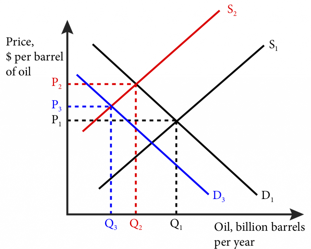
Panel b)
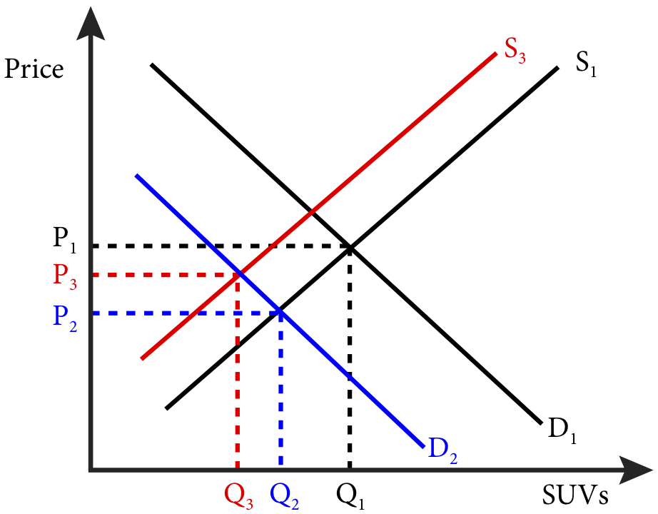
This drop in the price of SUVs will cause the automobile manufacturers to shift production away from SUVs and into more fuel-efficient compact cars and electric hybrids. This leads to a shift in SUV supply from S1 to S3 in panel b and the final price and quantity will be at P3 and Q3. Finally, this shift to more fuel efficient cars, along with other energy saving consumption changes will lower the demand for crude oil shifting the demand from D1 to D3 in panel a and resulting in a final price and quantity will be at P3 and Q3.
From this example we can see how markets that are connected influence each other in significant ways. When we ignore these linkages as we do in partial equilibrium analysis we can miss significant effects and our conclusions can be biased.
20.2 Trading Economy: Edgeworth Box Analysis
Learning Objective 20.2: Draw an Edgeworth box for a trading economy and show how a competitive equilibrium is Pareto efficient.
Though the two-market example introduces the idea of how equilibrium in one market adjusts to changes in another, it is still only a partial analysis. In this section we will build a simple economy from the most fundamental of starting places: the initial endowment of resources for members of the economy and we will then show how, through trade in the form of barter, they are able to make themselves better off. In fact, we will show how free trade will lead to a Pareto efficient outcome: one where it is not possible to make one person better off without hurting another person. In the next section we will add a currency prices and show how prices adjust to achieve equilibrium in the supply and demands of all individuals and show again that the outcome is Pareto efficient .
To start to construct our trading economy we need to start with in initial state of the world. To keep matters simple and tractable, our model will assume that there are only two people in this world and two resources. As with all such models in economics, the results are generalizable to many individuals and many goods.
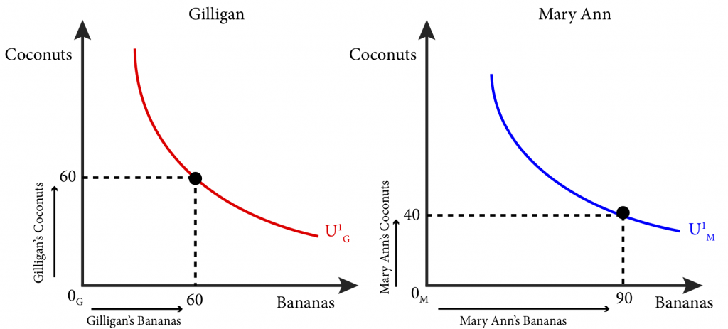
Imagine that two people from the same sea voyage are shipwrecked on two uninhabited tropical islands, separated by a small stretch of water – let’s call them Gilligan and Mary Ann. The only things the islands have for them to consume are the bananas and coconuts growing in the trees on both islands. Immediately after the shipwreck, they both take an inventory of the bananas and coconuts available to them. We call this initial allocation of goods their endowments. Gilligan finds that he has 60 coconuts and 60 bananas. Mary Ann has 40 coconuts and 90 bananas. The total amount of resources available to both of them is 100 (60+40) coconuts and 150 (60+90) bananas.
As in module 1 we can draw a graph for both Gilligan and Mary Ann that shows their initial bundle and their indifference curves through those bundles as in figure 20.2.1
Figure 20.2.1: Gilligan and Mary Ann’s Initial Endowments and Indifference Curves
The question for this module is, what happens when Gilligan and Mary Ann discover each other’s existence? More specifically, will they trade with each other and will it improve their well-being? To answer these questions we can begin by implementing a graphical technique called an Edgeworth Box (names after the English economist Francis Edgeworth) and shown in Figure 20.2.2. The Edgeworth box has dimensions that equal the total resources in the economy. In our case, its height is measured in coconuts and since there are 100 coconuts total, the height of the box is 100. The width of the box is measured in bananas and since there are 150 bananas in total, the width is 150. In this way the dimensions of the Edgeworth box represent the total endowment of the economy. We measure Gilligan’s resources from the origin in the southeast corner of the box, labeled 0G. In contrast, we measure Mary Ann’s resources from the northeast corner of the box, labeled 0M.
Figure 20.2.2: The Edgeworth Box for Gilligan and Mary Ann’s Economy
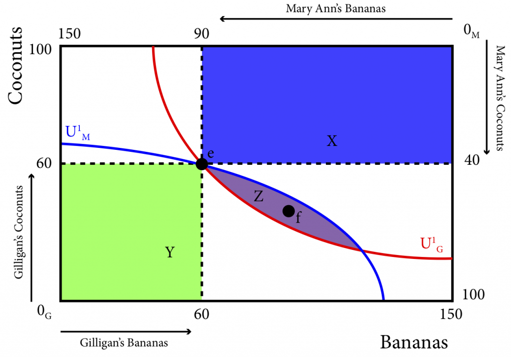
Now each of their initial endowments can be expressed by a single point, marked e. Note that at his point Gilligan has 60 coconuts. Since there are 100 coconuts in total, that leaves exactly 40 for Mary Ann. This is the distance from Gilligan’s 60 to the top of the box. We measure Mary Ann’s endowment of coconuts from the top of the box down to her endowment point, e. Her 40 coconuts, leaves 60 for Gilligan. The same is true for bananas: we measure Gilligan’s from left to right starting at 0G, and we measure Mary Ann’s bananas from right to left starting at 0M. In fact, any spot in the Edgeworth box represents a full distribution of all of the combined resources – this is the clever trick of the Edgeworth box. It also means that nothing is wasted, there are no left over resources available at any spot in the box.
As in Figure 20.2.1, we can draw indifference curves through the initial endowment point for both people. Gilligan’s is identical to the one in Figure 20.2.1. Mary Ann’s indifference curve is identical as well in relation to the new origin for her, 0M.
The trick to understanding the Edgeworth box is to imagine taking Mary Ann’s graph from Figure 20.1.1 and rotating it 180 degrees and then sliding it over until the endowment points for both are on the same spot. This is illustrated in Figure 20.2.3.
Figure 20.2.3: Creating the Edgeworth Box from Two Individual Initial Endowments and Indifference Curves

In the Edgeworth box in Figure 20.2.2, better consumption bundles for Gilligan are to the northeast of his initial indifference curve, U1G, or in the areas labeled X and Z, this is called the preferred set for Gilligan. Better bundles for Mary Ann are now to the southwest of her initial indifference curve, U1M, in the areas labeled Y and Z, the preferred set for Mary Ann. Note that area Z is the one area that is preferred set for both Gilligan and Mary Ann. This area Z is called the lens.
Now we have to ask the question, when Gilligan and Mary Ann become aware of each other and make contact, should they trade? Assuming nothing compels them to trade they will only engage in trade if they can be made better off because otherwise they will just keep their initial endowment. Assuming that Gilligan and Mary Jane are utility maximizers as usual, we have already identified a set of alternate distributions of resources that make the both better off, these are the feasible bundles in the lens. They are feasible because they represent a complete distribution of the available resources, as does any spot in the Edgeworth box. They make both people better off because they cause both to achieve a higher indifference cure and therefore higher utility. The movement from allocation e to allocation f is shown in Figure 20.2.4. Note that at f, both Gilligan and Mary Ann are on higher indifference curves: Gilligan moves from U1G to U2G, and Mary Ann moves from U1M to U2M. As long as there is a lens there is a mutually beneficial trade to be made, so only where the two indifference curves just touch each other, or are tangent to each other, does the lens disappear. One such point is point f.
Figure 20.2.4: Mutually Beneficial Trade to a Pareto Efficient Allocation
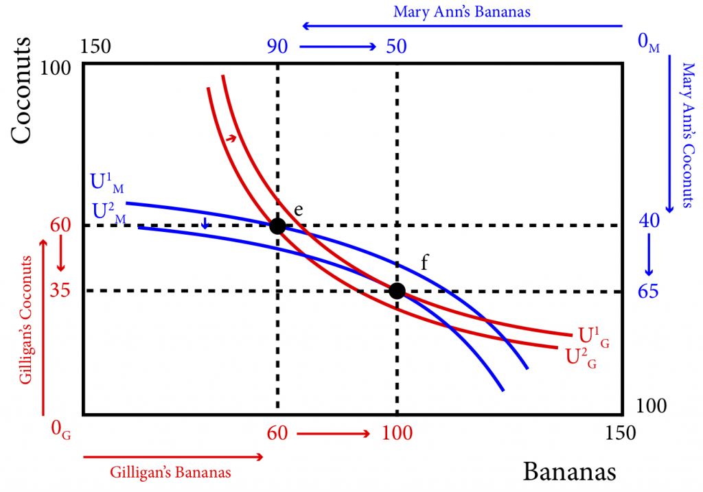
Point f isn’t just better for both, it is also Pareto efficient: there is no way to reallocate resources from that point without making one of the people worse off (on a lower indifference curve). So what is the trade that gets Gilligan and Mary Ann from e to f? Gilligan trades 25 coconuts to Mary Ann in exchange for 40 bananas. Gilligan goes from having 60 bananas to having 100 and from 60 coconuts to 35. Mary Ann goes from having 90 bananas to having 50 and from 40 coconuts to 65.
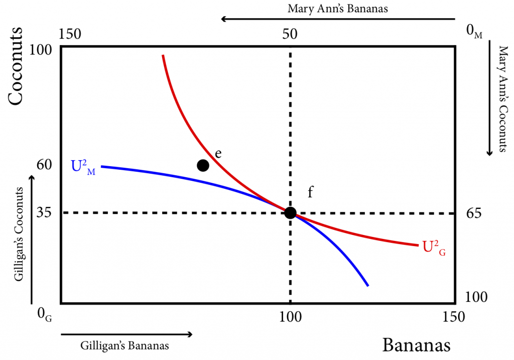
Why is point f both efficient and optimal? We know it is the point at which both Gilligan’s and Mary Ann’s indifference curves are tangent. This means that the marginal rates of substitution (MRS) of both are equal at f. Recall that the MRS of an agent is the rate at which they would trade one good for the other and be just as well off. When they are equal there is no more incentive to trade. For example if both parties are willing to trade one coconut for one banana, neither would be made better off trading.
NOTE: At the optimal bundle, MRSG=MRSM
On the other hand, if Gilligan could trade two coconuts for one banana and be just as well off (his MRS is 2) and Mary Ann could trade one coconut for two bananas and be just as well off (her MRS is ½), then if Gilligan traded one of his coconuts for one banana from Mary Ann it will make Gilligan better off (he only had to give up one coconut when he could give up two and be as well off) and Mary Ann better off (she only had to give up one banana when she could give up two and be as well off). This is similar to the situation at point e where Gilligan’s MRS is greater than Mary Ann’s MRS, so Gilligan trades coconuts for bananas.
Figure 20.2.5: At the Optimal Point the Indifference Curves are Tangent, the MRSs are Equal and the Allocation is Pareto Efficient.
But point f is not the only efficient allocation possible. In fact there are an infinite number of efficient allocations as the space is filled with an infinite number of indifference curves for both Gilligan and Mary Ann and therefore for each indifference curve for one person, there is a point of tangency with an indifference curve of the other. The contract curve is the line that connects all of these points of Pareto efficiency. Note that the contract curve begins and ends at the corners that represent the complete absence of goods for Gilligan, 0G, and Mary Ann, 0M. This is a Pareto efficient allocation as well because if Gilligan has nothing and Mary Ann has all of the coconuts and bananas, it is not possible to give Gilligan some without taking away from Mary Ann and making her worse off. The same logic applies at 0M.
Figure 20.2.6: The Contract Curve
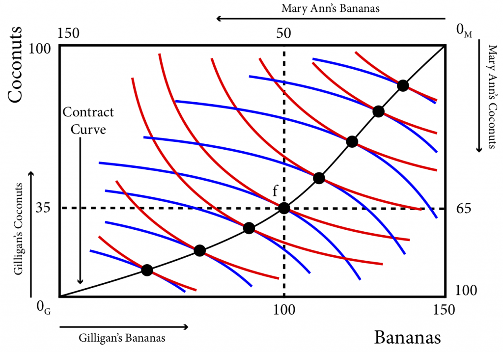
We know that there will always be an incentive to trade as long as the marginal rates of substitution are not equal and that from the initial allocation e they will trade to some point within the lens. We also know that f is a Pareto efficient allocation within the lens and is one such point. But the contract curve shows us that there are many Pareto efficient allocations in the lens. The portion of the contract curve that lies within the lens is the core and is shown in Figure 20.2.7.
Figure 20.2.7: The Contract Curve, the Lens and The Core
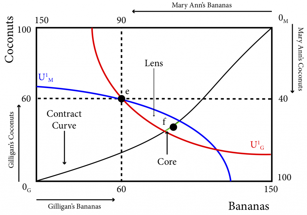
So, while we cannot predict precisely which allocation Gilligan and Mary Ann will end up on once they discover each other and decide to trade, we know that it will be somewhere on the core.
Note that through barter the individuals reach a Pareto efficient outcome but this outcome depends critically on the initial allocation. The initial allocation determines the lens or the range of possible outcomes given the initial allocation. Our policy example asks about tax and transfer schemes that address inequality. From this analysis it is clear that an unequal initial allocation will lead to outcomes that are also relatively unequal. So there is nothing within the barter economy that addresses or acts as a corrective for inequality.
The barter economy is a great introduction to general equilibrium and provides critical insight about how voluntary trade makes both parties better off and leads to Pareto efficient outcomes. However, in the real world most transactions do not happen by barter but through the use of money. In the next module we will expand our model to a competitive equilibrium setting with the use of money and where there are prices and consumers are price-takers.
MATHEMATICAL EXTENSION
We have described two conditions that define Pareto efficient allocations:
One, they are feasible. We have ensured feasibility with our graphical technique of the Edgeworth box – all allocations within the box are feasible.
Mathematically, a feasible allocation is one that meets the two following conditions:
[latex]\color{green}1)[/latex][latex]\color{green}b^G+B^M=B[/latex] , where B is the total amount of bananas and [latex]\color{green}b^G[/latex] is Gilligan’s share of bananas and [latex]\color{green}b^M[/latex] is Mary Ann’s share of bananas.
[latex]\color{green}2)[/latex] [latex]\color{green}c^G+c^M=C[/latex], where C is the total amount of coconuts and [latex]\color{green}c^G[/latex] is Gilligan’s share of bananas and [latex]\color{green}c^M[/latex] is Mary Ann’s share of coconuts.
Two, at Pareto efficient allocations the marginal rates of substitution are equal.
Mathematically the Marginal Rate of Substitution is:
[latex]\color{green}MRS^G=-\frac{MU\frac{G}{B}}{MU\frac{G}{C}}=-\frac{\frac{\partial U^G}{\partial b^G}}{\frac{\partial U^M}{\partial C^M}}[/latex], for Gilligan and
So the condition [latex]\color{green}MRS^G=MRS^M[/latex] is equivalent to:
[latex]\color{green}\frac{\frac{\partial U^G}{\partial b^G}}{\frac{\partial U^G}{\partial c^G}}=\frac{\frac{\partial U^M}{\partial b^M}}{\frac{\partial U^M}{\partial c^M}}[/latex]
Let’s consider a specific example. We have the total bananas (150) and coconuts (100) in the economy. Let [latex]\color{green}U^G-ln(B)+2ln(c)[/latex] and let [latex]\color{green}U^G=ln(B)+2ln(c)[/latex]
[latex]\color{green}\frac{\partial U^G}{\partial b^M}=\frac{1}{b^G}[/latex], and [latex]\color{green}\frac{\partial U^G}{\partial c^G}=\frac{2}{c^G}[/latex], so [latex]\color{green}\frac{\frac{\partial U^G}{\partial b^G}}{\frac{\partial U^G}{\partial c^G}}=\frac{c^G}{2b^G}[/latex]
[latex]\color{green}\frac{\partial U^M}{\partial b^M}=\frac{1}{b^M},and\,\frac{\partial U^M}{\partial C^M}=\frac{2}{c^M},so\frac{\frac{\partial u^M}{\partial b^M}}{\frac{\partial U^M}{\partial c^M}}[/latex]
[latex]\color{green}MRS^G=MRS^M\,is\,equivalent\,to\,\frac{c^G}{2b^G}=\frac{c^M}{2b^M}\,,or\,\frac{c^G}{b^G}=\frac{c^M}{b^M}[/latex] (19.2.1)
Now lets return to our feasibility constraints: [latex]\color{green}b^G+b^M=B[/latex] and [latex]\color{green}c^G+c^M=C[/latex]. Given our resources these become:
[latex]\color{green}b^M=150-b^G[/latex]
[latex]\color{green}c^G+c^M=100[/latex], or:
Substituting equations (14.2.2) and (14.2.3) into (19.2.1) yields the following expression of the tangency condition:
[latex]\color{green}c^G=\frac{2}{3}b^G[/latex]
This is the equation of the contract curve. In this simplified example, the contract curve is just the diagonal of the rectangular Edgeworth box.
20.3 Competitive Equilibrium: Edgeworth Box With Prices
Learning Objective 20.3: Demonstrate how prices adjust to create a competitive equilibrium that is Pareto efficient form any initial allocation of goods.
Much of the trade in the real world occurs in markets that use some sort of currency as the medium of exchange and where the prices are posted. Take, for example, a supermarket where food and other goods are displayed on shelves with prices listed. There is no bargaining; you either buy or you don’t buy a good at the price shown. To make our simple model more realistic we need to add a market and prices. The idea that two people stranded on tropical islands would consider themselves to be price takers might seem a little odd but we will maintain this assumption to keep the analysis simple. In reality we are applying this model to situations where there are many buyers and sellers – for example, think of a large farmer’s market where there are many different sellers of the same produce and many buyers as well.
So now, instead of exchanging bananas for coconuts, Gilligan and Mary Ann exchange them for Dollars. For example if Mary Ann wants more coconuts, she has to sell some bananas to earn money and then use the money earned to buy coconuts. With only two goods it is the relative price that matters because it is the relative price that determines the rate of exchange. For example, if the price of bananas is $1 and the price of coconuts is $2 then the rate of exchange of bananas to coconuts is $1/$2 or ½. It takes two bananas to get one coconut. This is true if the price of bananas was $100 and the price of coconuts was $200 instead – it would still take two bananas to get one coconut.
To start, let’s consider the price of bananas of $1 and the price of coconuts of $2. At the initial distribution of goods, the bounty of Gilligan’s island is worth $180 ($1 per banana x 60 bananas + $2 per coconut x 60 coconuts) and the resources on Mary Ann’s island are worth $170 ($1 x 90 + $2 x 40).
Now suppose Gilligan would like to trade: he knows, because of the prices, that he can trade at a rate of two bananas for one coconut. He could for example sell all his bananas for $60 and then buy 30 coconuts with the money earned. This would leave him with 0 bananas and 90 coconuts. Alternatively he can sell 45 coconuts to buy 90 bananas and he could then have all 150 bananas on the two islands and it would leave him with 15 coconuts. He could also end up with any other bundle that represents a two for one trade of bananas and coconuts. This set of available bundles at these prices is illustrated in Figure 20.3.1, and called the price line.
Figure 20.3.1: The Initial Endowment and the Price Line
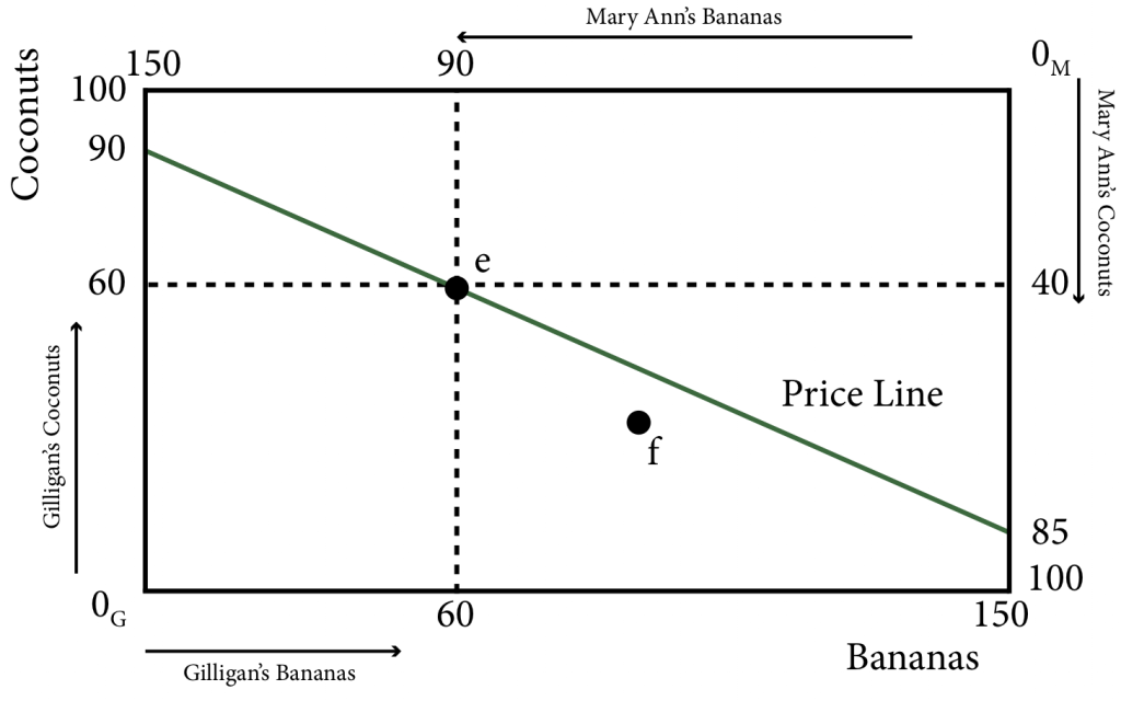
Mary Ann has equivalent choices, she can 90 bananas to earn $90 and then spend that money on 45 coconuts, leaving her with 0 bananas and 85 coconuts. Or she could sell 30 coconuts and buy 60 bananas leaving her with all 150 of the bananas on the two islands and 10 coconuts. Therefore the price line represents all the points in the Edgeworth box at which Gilligan and Mary Ann could end up, given the initial distribution of resources and the prices.
These prices do not allow Gilligan and Mary Ann to get to a Pareto efficient outcome however. Each of them maximizing their utility leads to two optimal bundles that are not feasible: together, they want too many bananas (more than the two islands have) and too few coconuts. This situation is shown in Figure 20.3.2.
Figure 20.3.2: No Equilibrium in the Product Markets
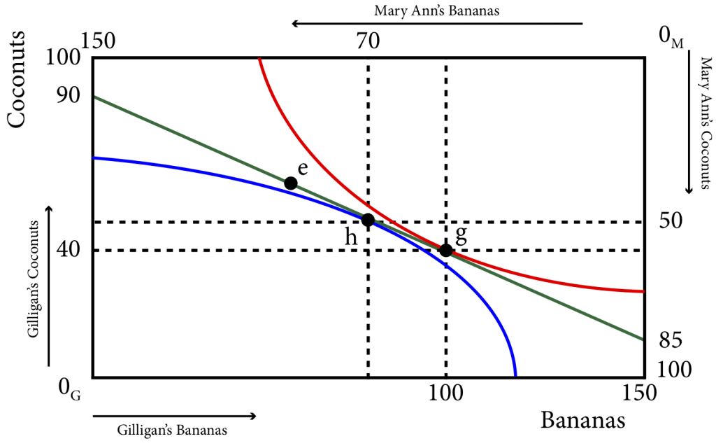
As we can see in Figure 20.3.2, Giligan’s optimal consumption bundle is at point g, where his indifference curve is tangent to the price line and Mary Ann’s optimal consumption bundle is at point h, where her indifference curve is tangent to the price line. At these bundles, Gilligan would like to consume 100 bananas and 40 coconuts and Mary Ann would like to consume 70 bananas and 50 coconuts. The total demand for bananas, 170 is greater than the total amount available, 150, and the total demand for coconuts, 90, is less than the total amount available, 100. Thus there is excess demand for bananas and excess supply of coconuts.
We know from previous modules that excess demand causes prices to rise and excess supply causes process to fall, so banana prices should rise, coconut prices should fall and therefore the relative price of bananas to coconuts should rise.
What is equilibrium in this market? Equilibrium is a set of prices, or a price ratio, where the number of bananas demanded by both Gilligan and Mary Ann exactly equals the total number available and the number of coconuts demanded by both Gilligan and Mary Ann exactly equals the total number available. In our case the price ratio [latex]\frac{PB}{Pc}=\frac{1.25}{2}[/latex] does exactly that.
Figure 20.3.3: Competitive Equilibrium in the Island Economy
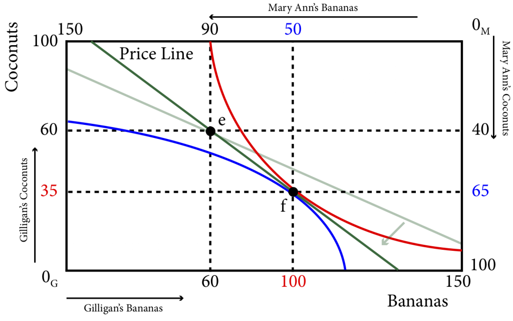
As can be seen in Figure 20.3.3, at the price ratio $1.25/$2, Gilligan wants to sell 25 coconuts at $2 a coconut, and with the $50 he earns from that sale he will buy 40 bananas at $1.25 a banana. At the same time Mary Ann wants to sell 40 bananas at $1.25 a banana and with the $50 she earns she wants to buy 25 coconuts. Equilibrium is achieved because the number of bananas Gilligan wants to buy is exactly equal to the number of bananas Mary Ann wants to sell and the number of coconuts Gilligan wants to buy is exactly equal to the number of coconuts Mary Ann wants to sell. Since this is the case the condition that characterizes the equilibrium point is:
[latex]MRS_G=-\frac{PB}{PC}=MRS_M[/latex]
In other words, both indifference curves and the price line all have the same slope at the optimal point, point f. This guarantees that the competitive equilibrium lies on the contract curve, which guarantees that it is Pareto efficient.
We call this result the First Theorem of Welfare Economics:
Any competitive equilibrium is Pareto Efficient
There is a second theorem that is closely related to the first. It concerns the ability of a social planner to select a particular equilibrium point along the contract curve. Is it possible to reallocate resources to achieve equilibrium at a desired point? The answer is yes.
Second Theorem of Welfare Economics:
Any Pareto Efficient competitive equilibrium is achievable through the reallocation of resources.
One implication of the second theorem is that society can address inequality through transfers of resources without any efficiency loss. Any efficient allocation on the contract curve can be achieved through a redistribution of the initial endowment. Note that this does not have to be on the contract curve but any initial endowment that lies on the equilibrium price line connecting the point on the contract curve.
MATHEMATICAL EXTENSION
We have described two conditions that define Pareto efficient allocations in an exchange economy in the previous section:
One, they are feasible, and two, the marginal rates of substitution are equal.
With a market economy with prices we now have to incorporate the price system into our analysis. What we know is that the price line connects the initial allocation and the equilibrium point: this means that the equilibrium has to be affordable and affordability is determined by the initial allocation and the prices themselves.
Let the initial allocation of bananas be given by [latex]\color{green}b^G+b^M=B[/latex], where B is the total amount of bananas and [latex]\color{green}b^G[/latex] is Gilligan’s share of bananas and [latex]\color{green}b^M[/latex] is Mary Ann’s share of bananas. The initial allocation of coconuts is given by [latex]\color{green}c^G+c^M=C[/latex], where C is the total amount of coconuts and [latex]\color{green}c^G[/latex] is Gilligan’s share of bananas and [latex]\color{green}c^M[/latex] is Mary Ann’s share of coconuts.
In terms of initial wealth, Giligan has:
[latex]\color{green}P_{b}b^{G}+p_cc^G[/latex]
This is how much Gilligan can earn from selling his endowment. Similarly MaryAnn has:
[latex]\color{green}P_bb^M+P_cc^M[/latex]
Any potential equilibrium has to be affordable, these affordability constraints are
where the hats on top of the b and the c represent equilibrium amounts. These constraints state that the total amount of money spent on the equilibrium allocations has to equal the amount earned from selling the initial allocation.
These constraints along with the equality of the marginal rates of substitution and the price ratio characterize the competitive equilibrium:
Note, however, that the nominal prices don’t matter at all, only relative prices matter since the nominal values do not affect the ability to exchange allocated goods for new goods. So we can set one price, pc, to $1.
Let’s consider the same specific example form the previous section. We have the total bananas (150) and coconuts (100) in the economy. Let [latex]\color{green}U^G=ln(B)+2ln(c)[/latex] and let [latex]\color{green}U^G=ln(B)+2ln(c)[/latex], we found that in equilibrium:
[latex]\color{green}MRS^G=MRS^M=P_b[/latex] is equivalent to [latex]\color{green}\frac{c^G}{2b^G}=\frac{c^M}{2b^M}=Pb[/latex] , or
[latex]\color{green}\frac{c^G}{b^G}=P_B[/latex]
And the contract curve is given as:
[latex]\color{green}c^G=\frac{2}{3}b^G[/latex] , or [latex]\color{green}c^G=\frac{2}{3}b^G,or\,\frac{c^G}{b^G}=\frac{2}{3}[/latex] .
Thus [latex]\color{green}\hat{P}b=\frac{2}{3}[/latex].
The demand functions for these Cobb Douglas type preferences are
[latex]\color{green}\hat{b}^G=\frac{50p_b+50}{P_b},and\,\hat{c}^G=\frac{\frac{1}{2}(50p_b+50)}{1}[/latex]
Thus the equilibrium quantities and prices are:
[latex]\color{green}\hat{b}^G=125[/latex]
[latex]\color{green}\hat{c}^G=42[/latex] (after rounding)
[latex]\color{green}\hat{b}^M=25[/latex]
[latex]\color{green}\hat{c}^M=58[/latex]
[latex]\color{green}\hat{p}_b=\frac{2}{3}[/latex]
[latex]\color{green}\hat{p}_c=1[/latex]
20.4 Production and General Equilibrium
Learning Objective 20.4: Draw a production possibility frontier and explain how the mix of production is determined in equilibrium and how productive efficiency is guaranteed.
In the example of desert island economies above we have ignored production – the bananas and coconut were simply there, endowed to the inhabitant of the island. Now we are going to add the final piece of complexity by adding production. Instead of a pile of coconuts and bananas available to the inhabitants, the inhabitants must produce them through the use of their labour to harvest them from trees on the islands. We will assume that both banana trees and coconut trees grow on both islands, but that Gilligan and Mary Ann differ in how many coconuts and bananas they can harvest in a day.
Banana trees are not tall and their fruit is easy to reach without climbing whilst coconut trees are very tall and require a lot of climbing to reach their fruit. It turns out that while they are both more than capable of harvesting both, Gilligan is more adept at finding and harvesting bananas while Mary Ann is relatively better at climbing trees and harvesting coconuts.
If Gilligan spends his entire day collecting coconuts he can collect 100, if he spends his entire day collecting bananas, he can collect 200. He can also split his time between the two activities. If we call β the fraction of his time he spends on banana harvesting, then 1-β is the time he spends on coconut harvesting. So in one day Gilligan will harvest 200 β bananas plus 100 (1-β) coconuts. By varying β from 0 to 1 we can find all the points in Gilligan’s Production Possibility Frontier: a line that shows all of the possible combinations of bananas and coconuts Gilligan can harvest in a single day. This is shown in panel a of Figure 20.4.1.
Figure 20.4.1: Individual Production Possibility Frontiers
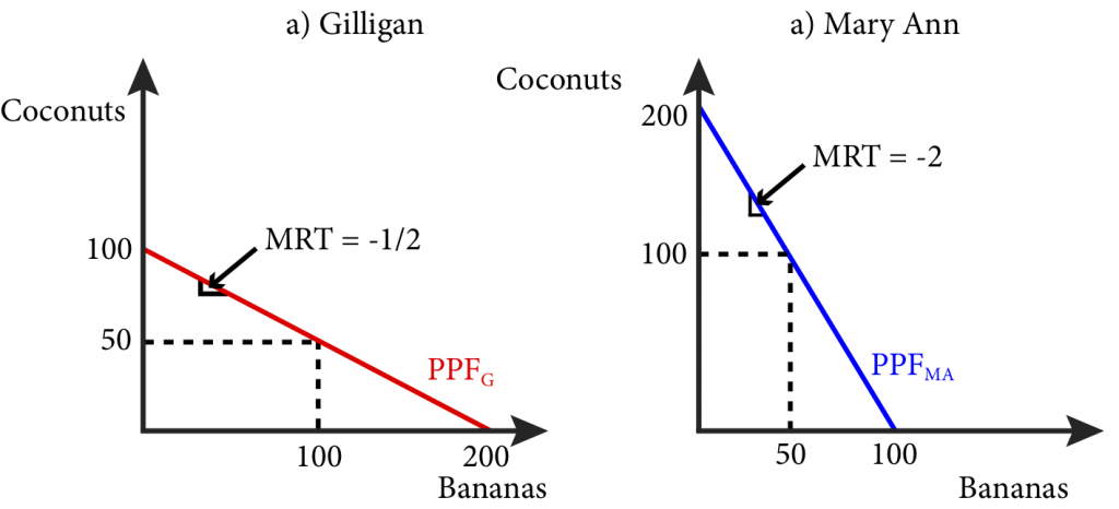
Similarly, if Mary Ann spends her entire day collecting coconuts she can collect 200, if she spends her entire day collecting bananas, she can collect 100. She can also split her time between the two activities. If we call β the fraction of his time she spends on banana harvesting, then 1-β is the time she spends on coconut harvesting. So in one day Mary Ann will harvest 100 β bananas plus 200 (1-β) coconuts. By varying β from 0 to 1 we can find all the points in Mary Ann’s Production Possibility Frontier. This is shown in panel b of Figure 20.4.1.
The slope of the production possibility frontier (PPF) is the Marginal Rate of Transformation (MRT): the cost of production of one good in terms of the foregone production of another good. This is the opportunity cost of producing that good. In this case the MRT is the amount of coconuts that can be collected if the collection of bananas is reduced by one banana. For Gilligan, every banana he chooses not to collect leads to enough time to collect ½ more coconuts, or put in another way, for every two bananas he gives up, he can collect one more coconut. Thus his MRT is -½ which is the same as the slope of his PPF. Similarly, for Mary Ann, if she reduces her banana collecting by one banana, she can collect 2 coconuts. So her MRT is -2 which is the same as the slope of her PPF.
This leads directly to the concept of Comparative Advantage: a person has a comparative advantage in the production of a good if they have a lower opportunity cost of production than someone else. In our case, Gilligan has a lower opportunity cost of producing (collecting) bananas as he gives up only ½ coconut per banana. It must be the case in this two good world that Mary Ann has a comparative advantage in collecting coconuts as she gives up only ½ a banana to collect a coconut (while Gilligan would have to give up 2). As the name suggests, this is a comparative concept, it is only relative to someone else. And it does not have anything to do with absolute productivity. To see this, suppose that Mary Ann could collect 1000 bananas and 2000 coconuts in a day. She would still have the same MRT, -2, and thus the same opportunity cost of bananas.
If they combined their outputs they would have a joint PPF as shown in Figure 20.4.2.
Figure 20.4.2: Joint Production
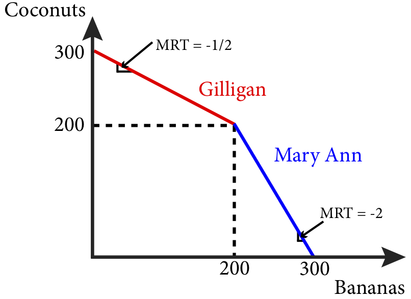
By producing based on their comparative advantage and trading both Gilligan and Mary Ann can be made better off. To see this imagine that both Gilligan and Mary Ann do not trade and spend half their time on each collecting activity. From Figure 20.4.1 we can see that Gilligan collects 100 bananas and 50 coconuts while Mary Ann collects 50 bananas and 100 coconuts. Now suppose that each spends all their time collecting the good in which they have a comparative advantage. Gilligan will collect only bananas and harvest 200 and Mary Ann will collect only coconuts and harvest 200. By sharing half their harvest with each other they will end up with 100 of each or 50 more in total. This is the lesson of trade based on comparative advantage: all parties can benefit.
As we add producers this adds segments to the PPF. For example suppose another person, whom we will call Thurston, arrives on the islands and his ability to collect bananas is 150 per day if he spends all his time collecting bananas and 150 coconuts if he spends his entire day collecting coconuts. Thurston’s PPF is shown in Figure 20.4.3.
Figure 20.4.3: Thurston’s Production Possibility Frontier
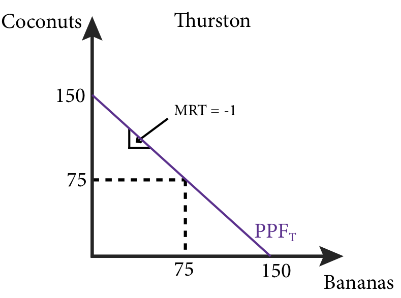
Thurston’s MRT is -1 and if he spends half his day collecting bananas and half his day collecting coconuts he will collect 75 of each.
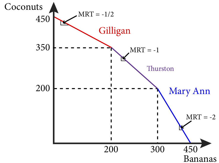
When we add Thurston’s PPF to the group, or joint production, PPF we have to think about the most effective way for the group to collect both bananas and coconuts. Starting from a position of all three spending their entire time collecting coconuts and thus collecting 450 coconuts and no bananas, we need to ask who is the best person to start collecting bananas if they want to add bananas to their collection. The answer, based on having the lowest opportunity cost, is Gilligan. But Gilligan can only collect 200 bananas if he devotes his entire day to the endeavor. What if the group wants to collect even more? The next best person is Thurston whose opportunity cost of collecting bananas is 1, which is lower than Mary Ann’s which is 2. Thus the second segment in the joint PPF is, therefore, Thurston’s PPF, followed by Mary Ann’s as is shown in Figure 20.4.4.
Figure 20.4.4: The Joint PPF with Thurston.
As we add more and more producers to this economy two things will happen. One, we will add their production to the joint PPF which will shift the PPF out as more goods are being produced overall, and two, we will add more and more segments of the joint PPF, each with their own slope and the joint PPF will become more and more smooth – the kinks in the curve will become less and less evident until eventually it will appear as a smooth curve as shown in green in Figure 20.4.5.
Figure 20.4.5: The Optimal Product Combination
The concave shape of the PPF leads to a MRT that is constantly changing. The slope becomes increasingly steeper as we move down the PPF and therefor the MRT increases in absolute value. The more bananas they produce the more coconuts they have to give up per banana. The MRT tells us the marginal cost of producing one extra banana in terms of the marginal cost of producing another good, in this case the MRT is the ratio of the marginal cost of bananas and the marginal cost of coconuts:
(20.1)
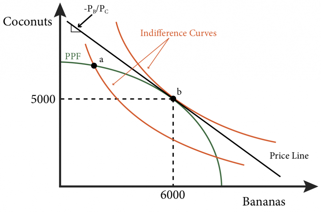
Every point on the PPF is both efficient, there are no wasted resources – production is at it maximum, and feasible. Now we want to know, which among all of the possible points should the actual production take place, what is the optimal mix of bananas and coconuts?
To answer this we need to know about the preferences of the consumers of the two goods. To keep things simple, assume that we can represent the preferences of every consumer in this economy with a single indifference curve, perhaps because every consumer has identical preferences. The optimal decision then is the point on the PPF that allows the consumers to achieve the highest indifference cure possible. In Figure 20.4.5, point b is on the PPF but leads to an indifference curve that is below the one that includes point a. Point a is the one point that allows the consumers the most utility from the product mix. It is also the one that is just tangent to the PPF at point a. This means that we have a familiar condition that characterizes the optimal mix of goods: MRS = MRT.
We know from Module 4 that utility maximizing consumers choose a bundle of good for which their marginal rate of substitution equals the slope of the budget line – the negative of the price ratio. If all consumers face the same price ratio, they will all pick a consumption bundle where they all have the same MRS. This is true even if their preferences differ because prices are common to all consumers and a condition of the optimal consumption bundle is that MRS equals the negative of relative prices. Because all consumers have the same MRS, no trades will happen, there are no mutually beneficial trades to be had. This is called consumption efficiency: it is not possible to redistribute goods to make one person better off without making another person worse off. This also indicates that the consumption bundle lies on the contract curve.
Suppose that, rather than being traded, bananas and coconuts are sold by competitive firms. In a perfectly competitive environment each firm sells a quantity of each good so that their marginal cost of production equals the price:
We divide one equation by the other to get:
(20.2)
From 14.1 we know that [latex]MRT=-\frac{MC_B}{MC_C}[/latex], so :
This has an intuitive explanation. Consider an MRT of -1, what this means is that the can trade off production one-for-one. They can produce one more banana by producing one less coconut. Now suppose that the price of bananas is $2 and the price of coconuts is $1 so the price ratio is -2. Should the firm adjust output? Yes. By producing one more banana they earn $2 more, they have to produce one less coconut to do so, but they only forgo $1 in earnings so their net gain is $1. Only where
Since we know the optimal consumption bundle is where MRS equals the negative of the price ratio, we know:
(20.4)
Equation 20.4 is illustrated in Figure 20.4.5 – the PPF, the price line and the indifference curves all have the same slope at point a. Competition ensures that MRT equals MRS and this means that the economy has achieved productive efficiency: there is no other mix of output levels that will increase the firm’s earnings.
We can combine the PPF and the Edgeworth box in the same graph by noting that each point on the PPF defines the dimensions of an Edgeworth box. In Figure 20.4.6, firms produce 150 bananas and 100 coconuts, point a on the PPF. This is the dimension of the Edgeworth box drawn inside of the PPF. The process that consumers pay are the same as the prices producers receive,
Figure 20.4.6: Competitive Equilibrium
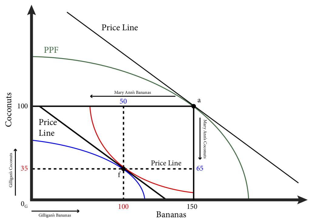
In equilibrium the price line is tangent to the consumers’ indifference curves at point f, as well as to the PPF at point a. Thus a competitive equilibrium is reached: consumers are maximizing their utilities at point f, producers are maximizing their returns at point a and supply equals demand in both markets: Gilligan consumes 100 bananas and 35 coconuts, Mary Ann consumes 50 bananas and 65 coconuts and the combines demand for both, 150 bananas and 100 coconuts exactly equals the supply.
SUMMARY
Review: Topics and Related Learning Outcomes
20.1 Partial Versus General Equilibrium
Learning Objective 20.1: Explain the difference between partial and general equilibrium.
20.2 Trading Economy: Edgeworth Box Analysis
Learning Objective 20.2: Draw an Edgeworth box for a trading economy and show how a competitive equilibrium is Pareto efficient.
20.3 Competitive Equilibrium: Edgeworth Box With Prices
Learning Objective 20.3: Demonstrate how prices adjust to create a competitive equilibrium that is Pareto efficient form any initial allocation of goods.
20.4 Production and General Equilibrium
Learning Objective 20.4: Draw a production possibility frontier and explain how the mix of production is determined in equilibrium and how productive efficiency is guaranteed.
Learn: Key Terms and Graphs
Terms
First Theorem of Welfare Economics
Second Theorem of Welfare Economics
Production Possibility Frontier
Marginal Rate of Transformation
Graphs
General Equilibrium in Oil and SUV markets
Gilligan and Mary Ann’s Initial Endowments and Indifference Curves
The Edgeworth Box for Gilligan and Mary Ann’s Economy
Creating the Edgeworth Box from Two Individual Initial Endowments and Indifference Curves
Mutually Beneficial Trade to a Pareto Efficient Allocation
The Contract Curve, the Lens and The Core
The Initial Endowment and the Price Line
No Equilibrium in the Product Markets
Competitive Equilibrium in the Island Economy
Individual Production Possibility Frontiers
Thurston’s Production Possibility Frontier
The Optimal Product Combination
Supplemental Resources
Examples
There are no supplemental YouTube videos for this module.
Policy Example
Policy Example: Should the Government Try to Address Growing Inequality Through Taxes and Transfers?
Learning Objective: Show how any redistribution of resources leads to a Pareto efficient competitive equilibrium.
Income inequality is the outcome of markets and society. An unequal distribution of societal resources can be represented in the abstract through the use of Edgeworth box analysis. Though an Edgeworth box represents only two people and two goods, the insight generalizes to many people and many goods. We can represent inequality by an initial distribution of societal resources that gives most of them to only one person as shown in Figure 1.
Figure 1: A Tax and Transfer Scheme to Address Initial Inequality
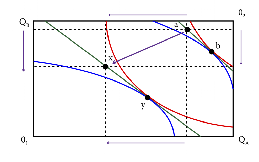
Figure 1 shows an economy where there are two people, 1 and 2, and two goods, A and B. The initial allocation is at a, where person 1 has most of both goods. The competitive equilibrium that obtains from this allocation is at b, which is still highly unequal. To address this, a tax and transfer scheme could be implemented by taking away some of the initial allocation of A and B from 1 and transferring them to 2. This is shown in the figure as the movement from allocation a to the allocation x. The government that does this is not able to know all of the societal preferences and thus is unable to know where the competitive equilibria are – they do not know the contract curve. So their tax and transfer scheme does not get them directly to a competitive equilibrium. However, the first and second welfare theorems ensure that the competitive equilibrium is Pareto efficient and that any Pareto efficient allocation can be obtained through a redistribution of the initial endowment.
So we can see in the figure that the new allocation x will lead to the Pareto efficient outcome y. This suggests that there is no efficiency loss from a tax and transfer scheme. Person 1 is worse off than before the taxes and transfers and person 2 is better off. Inequality has been addressed but whether society is better off because of it is something that would require additional analyses.
What we can say is that there are no wasted societal resources – there is no inefficiency. This assumes, however, that the tax and transfer scheme itself is costless while we know that in reality such a program would require a lot of bureaucratic costs. We also have not analyzed what a tax and transfer scheme would do to the incentive to produce. If the rich were not able to enjoy the full benefit of their labour because of an income tax, economic theory suggests that they might not work as hard and society would produce less. How would this reveal itself? In this case the PPF would shrink and so would the size of the Edgeworth box and since we assume more is better than the opposite must also be true – less is worse.
So both the bureaucratic costs and the loss from the dis-incentive to work suggests that there will be a cost to this program. The benefit is a more equal distribution of income. Thus whether it is a good idea to implement such a program depends on the relative benefits to a more equal income distribution and the costs of the program.
Candela Citations
- Authored by: Joel Bruneau & Clinton Mahoney. License: CC BY-NC-SA: Attribution-NonCommercial-ShareAlike
- Module 14: General Equilibrium. Authored by: Patrick Emerson. Retrieved from: https://open.oregonstate.education/intermediatemicroeconomics/chapter/module-14/. License: CC BY-NC-SA: Attribution-NonCommercial-ShareAlike
studying the changes in a single market in isolation
the study of how equilibrium is obtained in multiple markets at the same time
is the term for the initial allocation of goods
is the line on an Edgeworth box that connects all of the points of Pareto efficiency
is the portion of the contract curve on an Edgeworth box that lies within the lens
a theorem that states that any competitive equilibrium is Pareto Efficient
a theorem that states that any Pareto Efficient competitive equilibrium is achievable through the reallocation of resources
a line on a graph that shows all of the possible combinations of goods that can be produced in a given time frame
is the cost of production of one good in terms of the foregone production of another good; this is also the slope of the production possibility frontier
a person has a comparative advantage in the production of a good if they have a lower opportunity cost of production than someone else
occurs when it is not possible to redistribute goods to make one person better off without making another person worse off
occurs when there is no other mix of output levels that will increase the firm’s earnings
