
10
Joel Bruneau and Clinton Mahoney
Learning Objectives
- Derive the seven short-run cost curves from the total cost function
- Derive the three long-run cost curves from the total cost function
- Explain why long-run costs are always as low or lower than short-run costs and how more flexibility in choosing inputs is always better than less
- Explain how making more than one product, learning over time and learning by producing can lower costs
Module 9: Cost Curves
The Policy Question: Should the Federal Government Promote the Domestic Production of Streetcars?
In recent years, streetcars have enjoyed a bit of a renaissance in the U.S. Streetcars are electric powered public transit that ride on rails embedded into normal city streets and comingle with traffic. Once common in the U.S., and still common in many European cities, streetcars all but disappeared from U.S. streets in the second half of the 20th century. Portland, Oregon is one city that revived the streetcar and subsequently expanded their system.
After initially buying streetcars form the German company Siemens, Portland’s transit authority and government, pushed by the federal government, which funds a large portion of urban transit projects, decided to contract with a local firm, Oregon Iron Works to produce the streetcars locally. Oregon Iron Works had no experience in manufacturing streetcars, but created a subsidiary firm to do so called United Streetcar. Other U.S. cities that were introducing streetcars, such as Washington D.C. and Tucson, Arizona, contracted with Oregon Iron Works for their cars as well. In the end the firm faced severe delays and cost overruns and eventually got very behind on their scheduled delivery. In addition, the expected boom in streetcars slowed considerably with the recession of 2008 and changing municipal priorities. In 2014 United Streetcar ceased production and laid off its workers.
Source: Laris, Michael, “U.S. effort to help homegrown streetcar manufacturer falls short,” The Washington Post, November 29, 2014. http://www.washingtonpost.com/local/trafficandcommuting/us-effort-to-help-build-homegrown-streetcar-manufacturer-falls-short/2014/11/29/98c649b0-70b9-11e4-ad12-3734c461eab6_story.html
Exploring the Policy Question
Is the story of United Streetcar an example of a misguided effort to steer business domestically? Would it have succeeded if the market for streetcars in the U.S. had not dried up? To answer these questions we need to think about the cost structure of the industry and whether there are aspects of it that would support the decision to start manufacturing streetcars domestically. Cost curves—the subject of this module—are critical tools in analyzing a company’s cost structure.
9.1 Short-Run Cost Curves
Learning Objective 9.1: Derive the seven short-run cost curves from the total cost function.
9.2 Long-Run Cost Curves
Learning Objective 9.2: Derive the three long-run cost curves from the total cost function.
9.3 Short-Run Versus Long-Run Costs: The Advantage of Flexibility
Learning Objective 9.3: Explain why long-run costs are always as low or lower than short-run costs and how more flexibility in choosing inputs is always better than less.
9.4 Multiproduct Firms, Learning Curves, and Learning-by-Doing
Learning Objective 9.4: Explain how making more than one product, learning over time and learning by producing can lower costs.
9.1 Short-Run Cost Curves
LO 9.1: Derive the seven short-run cost curves from the total cost function.
A cost curve represents the relationship between output and the different cost measures involved in producing the output. Cost curves are visual descriptions of the various costs of production. In order to maximize profits firms need to know how costs vary with output, so cost curves are vital to the profit maximization decisions of firms.
There are two categories of cost curves: short-run and long-run. In this section we focus on short-run cost curves.
The Seven Short-Run Cost Measures
The short-run, as we learned in the previous module, is a time period short enough that some inputs are fixed while others are variable. There are seven cost curves in the short-run: fixed cost, variable cost, total cost, average fixed cost average variable cost, average total cost and marginal cost.
The fixed cost (FC) of production is the cost of production that does not vary with output level. The fixed cost is the cost of the fixed inputs in production, such as the cost of a machine (capital) that costs the same to operate no matter how much production is happening. An example of such a machine is a conveyor belt in a factory that moves a streetcar chassis through various stages of an assembly line. The belt is either on or off, but the cost of running it does not change depending on how many streetcars it carries at any point in time.
Note that the fixed cost of a piece of capital equipment that the company owns includes the opportunity cost as well. In our example, the fixed cost includes the actual costs of running the conveyer belt, such as power and maintenance, as well as the opportunity cost of using it for the firm’s own production rather than renting it out to another company.
The variable cost (VC) of production is the cost of production that varies with output level. This is the cost of the variable inputs in production, for example the cost of the workers that assemble the electronic devices along a conveyor belt. The number of workers might depend on how many devices the factory is trying to produce in a day. If its production target increases, it uses more labour. Thus the hourly wages it pays for these workers are a variable cost. Variable cost generally increases with the amount of output produced.
Like fixed cost of production, there is an opportunity cost associated with variable cost of production. In this case, the next best alternative use of these workers is to go to another firm that will employ them. Thus the market wage for workers represents their opportunity cost, and as such, the wage cost of employing them is equivalent to their opportunity cost.
The total cost (C) of production is the sum of fixed and variable costs of production:
There are three short-run average cost measures: the average variable cost, average fixed cost and average total cost.
Average variable cost (AVC) is the variable cost per unit of output. Mathematically, it is simply the variable cost divided by the output:
AVC = VC/Q
Note that since variable cost generally increases with the amount of output produced, the average variable cost can increase or decrease as output increases.
Average fixed cost (AFC) is the fixed cost per unit of output. Mathematically, it is simply the fixed cost divided by the output:
AFC = FC/Q
Because fixed cost does not change with the amount of output produced, the average fixed cost always decreases as output increases.
Average total cost (AC), or simply average cost, of production is total cost per unit of output. This is the same as the sum of the average fixed cost and the average variable cost:
AC = AC/Q = AFC + AVC
Because it is the sum of the average fixed cost, which is always declining with output, and the average variable cost, which may increase or decrease with output, the average total cost may increase or decrease with output.
Marginal cost (MC) is the additional cost incurred from the production of one more unit of output. Thus marginal cost is:
The only part of total cost that increases with an additional unit of output is the variable cost, so we can re-write the marginal cost as:
CALCULUS APPENDIX:
The marginal cost is the rate of change of the total cost as output increases, or the slope of the total cost function, C(Q). To find this we need to simply take the derivative of the total cost function:
[latex]\color{green}MC(Q)=\frac{dC(Q)}{dQ}[/latex]
Since [latex]\color{green}C(Q)=FC+VC(Q)[/latex] we can rewrite this derivative as: [latex]\color{green}MC(Q)=\frac{dFC}{dQ}+\frac{dVC(Q)}{dQ}[/latex]
FC is a constant so [latex]\color{green}\frac{dFC}{dQ}=0[/latex]. Thus
[latex]\color{green}MC(Q)=\frac{dVC(q)}{dQ}[/latex]
Since fixed cost does not change as output increases, marginal cost depends only on the variable cost.
Fixed Cost, Variable Cost, and Total Cost Curves
Table 9.1.1 summarizes a firm’s daily short-run costs. The firm has a fixed cost of $50 per day of production. This cost is incurred whether the firm produces or not, as we can see by the fact that $50 is still a cost when output is zero. The firm’s fixed cost of $50 does not change with the amount of output produced. The data in the first two columns of Table 9.1.1 allow us to draw the firm’s fixed cost curve. It is a horizontal line at $50, as shown in Figure 9.1.1.
Table 9.1.1: An Example of the Seven Short-Run Cost Measures
|
Output |
Fixed Cost |
Variable Cost |
Total Cost |
Marginal Cost |
Average Fixed Cost |
Average Variable Cost |
Average Cost |
|
Q |
FC |
VC |
C |
MC |
AFC |
AVC |
AC |
|
0 |
50 |
0 |
50 |
– |
– |
– |
– |
|
1 |
50 |
40 |
90 |
40 |
50.0 |
40.0 |
90.0 |
|
2 |
50 |
70 |
120 |
30 |
25.0 |
35.0 |
60.0 |
|
3 |
50 |
90 |
140 |
20 |
16.7 |
30.0 |
46.7 |
|
4 |
50 |
100 |
150 |
10 |
12.5 |
25.0 |
37.5 |
|
5 |
50 |
120 |
170 |
20 |
10.0 |
24.0 |
34.0 |
|
6 |
50 |
150 |
200 |
30 |
8.3 |
25.0 |
33.3 |
|
7 |
50 |
190 |
240 |
40 |
7.1 |
27.1 |
34.3 |
|
8 |
50 |
240 |
290 |
50 |
6.3 |
30.0 |
36.3 |
|
9 |
50 |
300 |
350 |
60 |
5.6 |
33.3 |
38.9 |
|
10 |
50 |
370 |
420 |
70 |
5.0 |
37.0 |
42.0 |
Figure 9.1.1: Three short-run cost curves – fixed, variable and total costs.
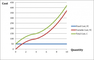
Figure 9.1.1 also shows variable and total cost curves plotted from data in Table 9.1.1. The variable cost increases with output, because extra output requires extra variable inputs. As we can see in the graph, the variable cost curve rises as output, Q, increases.
The short-run variable cost curve is determined by and matches the shape of the short-run production function, which we studied in Module 7. The short-run production function is the same as the total product of labour curve when labour is the variable input in the short-run, which we always assume it is. To go from the production function to the variable cost curve requires knowing the price of labour. Let’s assume a constant price of labour, say $10 an hour.
Figure 9.1.2 presents a typical short-run production function which leads to the shape of the variable cost curve in figure 9.1.1. The production function exhibits increasing marginal returns to labour initially: as the labour input is increased from zero the output increases at an increasing rate. Eventually however, the addition of extra hours of labour leads to additional output at a decreasing rate. This happens as we increase labour input from 10 hours of labour.
Figure 9.1.2: The Total Product of Labour Curve
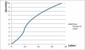
If we multiply the amount of labour at every level of output in Figure 8.1.2 by the wage rate of $10 per hour we get the variable cost curve from Figure 9.1.1
Marginal, Average Fixed, Average Variable and Average Total Cost Curves
Figure 9.1.3 presents the four remaining short-run cost curves: marginal cost (MC), average fixed cost (AFC), average variable cost (AVC) and average total cost (AC).
Figure 9.1.3: Short-Run Marginal Cost, Average Fixed Cost, Average Variable Cost, and Average Total Cost Curves.
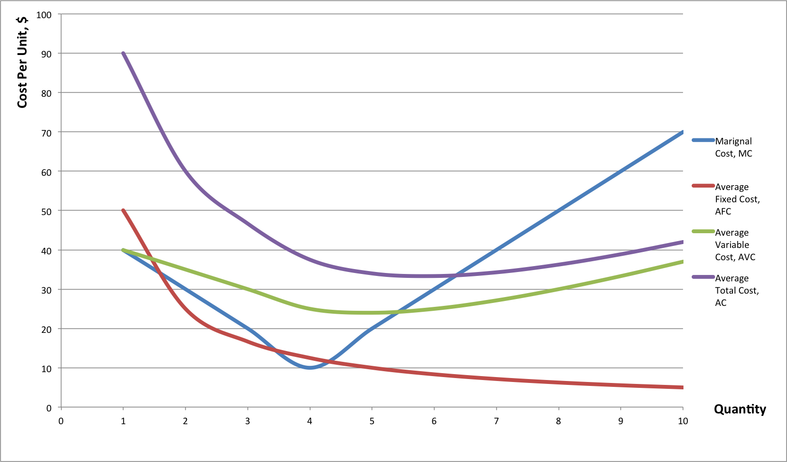
The marginal cost, average variable cost, and average total cost curves are derived from the total cost curve.
From Figure 9.1.3 you can see that the marginal cost curve crosses both the average variable cost curve and the average fixed cost curve at their minimum points. This is not random. Since the marginal cost indicates the extra cost incurred from the production of the next unit of output, if this cost is lower than the average, it must be bringing the average down. If this cost is higher than the average, it must pull the average up. Think of your own grade point average: if your average this term is higher than your overall average, your overall average will go up. If your average this term is lower than your overall average, your overall average will go down.
Calculus MEL
- If the total cost curve of a firm is C(Q) = 25+10Q2
- What is the marginal cost curve?
- What is marginal cost at Q=125?
9.2 Long-Run Cost Curves
LO 9.2: Derive the three long-run cost curves from the total cost function.
As we learned in previous modules, in the long run all inputs are variable and there are no fixed costs. In this section we look at the three long-run cost curves–total cost, average cost, and marginal cost—and how to derive them.
To determine the long run total cost (LRTC) for a firm we must think about the cost minimization problem, introduced in Module 8. Remember that the cost minimization problem answers the question: what is the most cost effective way to produce a given amount of output? The total cost curve represents the cost associated with every possible level of output, so if we figure out the cost minimizing choice of inputs for every possible level of output we can determine the cost of producing each level of output.
When we do this exercise we are looking for the expansion path of the firm. Recall from Module 8 that the expansion path is the combination of inputs that minimize costs for every level of output, and it can be graphed as a curve. Figure 9.2.1 shows the expansion path for a firm that manufactures tablet computers.
Figure 9.2.1: Expansion Path
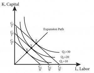
Each point on the expansion path is the solution to the cost minimization problem for that particular output. Recall from Module 8 that r is the rental rate or price of capital and w is the wage rate or price of labour. Consider point X: here the output quantity is set at 10 million and the tangency of the isocost and isoquant at this point establishes the optimal combination of the inputs. To go from this point to the cost we have only to know the combined cost of the inputs at this point. Fortunately, the isocost line at this point tells us exactly that, the total cost here is C1. Now consider point Y where output quantity has increased to 20 million. With this new production level is associated a new isocost curve with total cost at C2. Finally, point Z indicates that for an output quantity of 30 million the total cost is C3.
From the expansion path we can draw the total cost curve. We have three points already, X, Y and Z. Point X describes a quantity of 10 million tablets and a total cost of C1. Point Y describes a quantity of 20 million tablets and a total cost of C2. Point Z describes a quantity of 30 million tablets and a total cost of C3. These three cost-quantity pairs are three points on the long run total cost curve illustrated in figure 8.2.2.
Figure 9.2.2: The Long Run Total Cost Curve

Remember from Module 8 that the total cost is the sum of the input costs, LRTC = wL+rK. As we expand output we must use more inputs and the increase in labour and capital results in increasing overall cost of production.
Long-Run Average and Marginal Cost Curves
A firm’s long-run average cost (LRAC) is the cost per unit of output. In other words it is the total cost, LRTC, divided by output, Q:
A firm’s long-run marginal cost (LRMC) is the increase in total cost from an increase in an additional unit of output:
[latex]LRMC(Q)=\frac{\Delta LRTC(Q)}{\Delta Q}[/latex]
Where ∆LRTC(Q) is the change in total cost and ∆Q is the change in output. This is the same thing as the slope of the total cost curve, LRTC(Q).
CALCULUS APPENDIX
The long-run marginal cost is the rate of change of the total cost as output increases, or the slope of the total cost function, LRTC(Q). To find this we need to simply take the derivative of the total cost function:
[latex]\color{green}LRMC(Q)=\frac{dLRTC(Q)}{dQ}[/latex]
Figure 9.2.3 illustrates the relationship between the total cost curve (panel a) and the average and marginal cost curves (panel b).
Figure 9.2.3: Deriving Long-Run Average and Marginal Cost Curves from the Long-Run Total Cost Curve
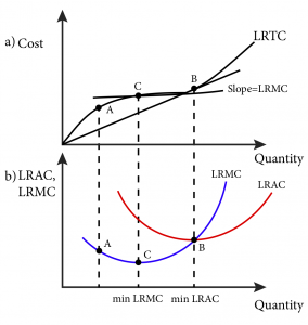
To see how long-run total and average costs are related, take point A on the total cost curve in Figure 9.2.3. At this point we can derive the average cost by dividing the vertical distance, which gives us the total cost, by the horizontal distance, which gives us quantity. This is the same thing as the slope of the ray from the origin that connects to point A: it is the ‘rise’ over the ‘run.’ So in panel b, we have the same quantity on the horizontal axis but the slope of the ray connecting to point A, or the average cost, on the vertical axis. Point A is, therefore, a point on the average cost curve. Note that as we move out along the total cost curve the ray from the origin to the total cost curve becomes less and less steep until the point B, after which the slope gets steeper. Thus the point B is the point of minimum average cost as illustrated in panel b.
To understand the relationship between long-run total cost and marginal cost let’s go back to point A in panel a. The marginal cost is the same as the slope of the total cost curve and we can illustrate the slope by using a tangent line: a straight line that passes through point A and has the same slope as the curve at that point. This slope gives us the marginal cost. Note that this slope is not as steep as the ray from the origin that defined average cost at this point. Therefore in panel b the marginal cost is lower than the average. We can also observe that as we move along the total cost curve the slope continues to decrease until point C after which the slope begins to increase. Thus point C is the minimum marginal cost as illustrated on the marginal cost curve in panel b.
Finally, note that at point B on the total cost curve the slope of the ray from the origin and the slope of the total cost curve are identical. At this point the marginal and the average costs are the same as seen by the intersection of the two curves in panel b.
This relationship between average and marginal costs is not a coincidence; it is always true. When average cost is above marginal cost, average cost must be decreasing. When average cost is lower than marginal cost, average cost must be increasing. And when average and marginal cost are equal, average cost is not changing. This relationship is described in Table 9.2.1 and illustrated in Figure 9.2.4.
Table 9.2.1 The Relationship between Long-Run Average and Marginal Costs
|
Relationship between AC and MC |
Resulting change in AC |
|
AC(Q)>MC(Q) |
AC(Q) increasing |
|
AC(Q)<MC(Q) |
AC(Q) decreasing |
|
AC(Q)=MC(Q) |
AC(Q) constant |
Figure 9.2.4: Relationship Between the Long-Run Average and Marginal Cost Curves
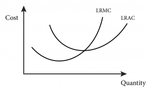
On the left half of figure 9.2.4 the average cost is above the marginal cost and thus the average cost is falling. On the right half of figure 9.3.4 the average cost is below the marginal cost and thus the average cost is rising. At the intersection of the two curves the average cost is at it minimum and the slope of the average cost curve is zero.
Economies and Diseconomies of Scale
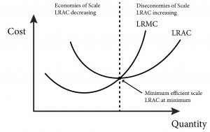
An important economic concept associated with the long-run average cost curve is economies of scale. Economies of scale occur when the average cost of production falls as output increases. Similarly, diseconomies of scale occur when the average cost of production rises as output increases. In a typical long-run average cost curve there are sections of both economies of scale and diseconomies of scale. There is also a point or region of minimum efficient scale where average cost is at its minimum. This is the point where economies of scale are used up and no longer benefit the firm. Figure 9.2.5 illustrates these points.
Figure 9.2.5: Economies, Diseconomies and Minimum Efficient Scale
9.3 Short-Run Versus Long-Run Costs: The Advantage of Flexibility
LO 9.3: Explain why long-run costs are always as low or lower than short-run costs and how more flexibility in choosing inputs is always better than less.
Short-run average costs are constrained by the presence of a fixed input. So in the long run we can always do at least as well as, and often better than, in the short run with respect to cost. We can see this is true by comparing the long-run and short-run average cost curves.
The long-run average cost curve is a type of lower boundary of the short-run cost curves. This can be understood most easily by thinking of a series of short-run average total cost curves, each one for a different level of the fixed input, capital, as shown in Figure 9.3.1.
Figure 9.3.1: The Long-Run Average Cost Curve as the Lower Boundary of Short-Run Average Cost Curves.
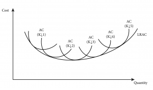
Since capital is variable in the long run, the long-run average cost is essentially the same as picking among the short-run average total cost curves and combining the capital with the optimal level of labour, or in other words, the minimum ATC.
The long run average cost curve illustrates the benefit of flexibility: by being able to choose both inputs the firm can ensure the efficient mix of the inputs is being used at all times which keeps costs at their minimum points for all output levels. This flexibility means that we can expect that in the long run, the average cost of production is at least as low as, and generally lower than in the short-run.
9.4 Multiproduct Firms and Learning Curves
LO 9.4: Explain how making more than one product, learning over time and learning by producing can lower costs.
A number of other factors matter in a firm’s ability to lower costs. In this section we look at two of them.
Multiproduct Firms
Often, a firm will make more than one product. This raises the interesting question, when is it better for the same firm to make multiple products than for multiple firms to each make one product. One answer lies in the concept of economies of scope: An economy of scope exists when the average cost of one product falls as the production of another product increases.
Take for example a firm that makes large LCD televisions. One expensive component of these displays is the flat glass panels needed for the screen. To make these large screens, very large pieces of glass are manufactured and then cut into individual rectangular pieces for the televisions. Often there are smaller glass pieces left over. Rather than discard these pieces, the same company can make smaller LCD displays for computers, cars, appliances and so on. Since a lot of the other materials, technical know-how, skilled labour and the like can be shared across the two types of products, the average cost of both declines when the production of smaller LCD displays for computers is increased.
More formally, we can think of a multiproduct firm as having a cost function that depends on the output of two goods: Q1 and Q2. Such a cost function can be expressed as C(Q1, Q2). We say the economies of scope are present if:
C(Q1, Q2) < C(Q1, 0) + C(0, Q2)
This equation makes intuitive sense. The left hand side of the inequality is the cost of a single firm that produced positive quantities of both goods. The right hand side is the total cost of producing only Q1 added to the total cost of producing only Q2. If it is cheaper to produce the two together then the inequality holds.
Learning Curves
Sometimes firms get better at making things over time, as they gain experience. Economists call this learning-by-doing Learning by doing means that as the cumulative output–the total output ever produced–of the firm increases the average cost falls.
Learning by doing can take different forms:
- Over time workers become more efficient at specific tasks they perform repeatedly.
- Managers can observe production and adjust task assignments and other aspects of the production process.
- Engineers can optimize product and plant design to increase efficiency.
- Firms can get better at handling inputs, materials and inventories.
These and other instances of learning by doing often lower firms’ average costs and make them more efficient over time.
The idea of learning by doing can be graphed as a learning curve (Figure 9.4.1) where average cost is plotted as a function of either time or cumulative output. The learning curve is different from the typical average cost curve, which represents the total cost divided by current output.
Figure 9.4.1: The Learning Curve
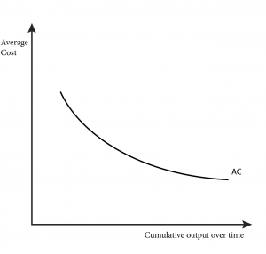
This temporal view of average costs makes firms’ decisions about operating and investing in the business more complicated. If a firm that is considering shutting down in the face of negative economic profits expects that they will be able to produce more efficiently in the future, they might be willing to accept near-term losses in the expectation of future profits.
The learning curve is potentially important in the policy question. If there is substantial learning involved in the production of a streetcar then the domestic manufacturer of streetcars might see its production costs decrease significantly as they produce more and more streetcars. So, although the short-run costs of production might suggest that domestic promotion is a bad idea, if there is good reason to believe that in the long-run average costs will decrease significantly, a reasonable case could be made for such promotion.
SUMMARY
Review: Topics and Related Learning Outcomes
9.1 Short-Run Cost Curves
Learning Objective 9.1: Derive the seven short-run cost curves from the total cost function.
9.2 Long-Run Cost Curves
Learning Objective 9.2: Derive the three long-run cost curves from the total cost function.
9.3 Short-Run Versus Long-Run Costs: The Advantage of Flexibility
Learning Objective 9.3: Explain why long-run costs are always as low or lower than short-run costs and how more flexibility in choosing inputs is always better than less.
9.4 Multiproduct Firms, Learning Curves, and Learning-by-Doing
Learning Objective 9.4: Explain how making more than one product, learning over time and learning by producing can lower costs.
Learn: Key Terms and Graphs
Terms
Graphs
Three short-run cost curves – fixed, variable and total costs
The Total Product of Labour Curve
Marginal Cost, Average Fixed Cost, Average Variable Cost, and Average Total Cost
Deriving Long-Run Average and Marginal Costs Curves from the Long-Run Total Cost Curve
Relationship Between the Long-Run Average and Marginal Cost Curves
The Long-Run Average Cost Curve as the Lower Boundary of Short-Run Average Cost Curves
Equations
Supplemental Resources
Practice Questions
YouTube Videos
These videos from the YouTube channel ‘Department of Economics’ may be helpful.
Policy Example
Policy Example: Should the Federal Government Promote the Domestic Production of Streetcars?
Learning Objective: Use an analysis of costs to explain why building streetcars domestically in the U.S. is or is not a good policy.
To understand the business of building streetcars we must first think about the cost structure. Streetcars are large, heavy and loaded with specific and sophisticated technology, such as electric propulsion engines, car electronics and controls, and passenger controls. Their manufacture takes a factory of considerable size and yet they are produced in small quantities. This suggests a few things about their costs:
- There are very large fixed costs because of the machinery and plant required for constructing these cars. Because of this the minimum efficient scale is probably far beyond any one manufacturer’s current scale. What this means is that the more streetcars a manufacturer produces, the lower the cost per car.
- Because of the complexity, there are likely to be large cost savings over time as a result of learning-by-doing.
- The complexity of the streetcar itself suggests that the quality of the product from new firms might suffer because they have not had the experience that long-time suppliers have had.
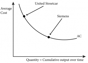
These observations suggest that current suppliers of streetcars, like Siemens, have considerable cost advantages over new firms because of their current production level that allows them to take advantage of economies of scale and because they are much farther along the learning curve (see Figures 1 and 2). Any new firm likely would take a very long time to reach both the scale efficiencies and the cost efficiencies from learning-by-doing of the current manufacturers. However, if the demand for streetcars was expected to grow and be sustained for a long period of time, a reasonable case could be made that the domestic industry could mature into a reliable and cost efficient supplier of streetcars to the U.S. and even international market.
Figure 1: Streetcar Manufacturers on the Long Run Average Cost Curve
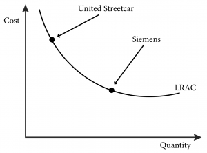
Figure 2: Streetcar Manufacturers on the Learning Curve
Unfortunately, the projections of the level of demand for streetcars appear to have been far too optimistic. It seems unlikely that the domestic streetcar industry will have a chance to grow and learn, so we may never know if it would have become cost competitive over time.
Exploring the Policy Question
1) Because of their size and weight, shipping streetcars internationally is costly. How would you include transportation costs in your analysis of the policy question?
2) If the market had not dried up, do you think United Streetcar would have succeeded in the long-run? Why or why not? Use economic reasoning in your answer.
Candela Citations
- Authored by: Joel Bruneau & Clinton Mahoney. License: CC BY-NC-SA: Attribution-NonCommercial-ShareAlike
- Module 8: Cost Curves. Authored by: Patrick Emerson. Retrieved from: https://open.oregonstate.education/intermediatemicroeconomics/chapter/module-8/. License: CC BY-NC-SA: Attribution-NonCommercial-ShareAlike
- Myriad Costs. Authored by: Preston McAfee & Tracy R Lewis. Retrieved from: https://resources.saylor.org/wwwresources/archived/site/textbooks/Introduction%20to%20Economic%20Analysis.pdf. License: CC BY-NC-SA: Attribution-NonCommercial-ShareAlike
represents the relationship between output and the different cost measures involved in producing the output
of production is the cost of production that does not vary with output level; the fixed cost is the cost of the fixed inputs in production, such as the cost of a machine (capital) that costs the same to operate no matter how much production is happening
of production is the cost of production that varies with output level. This is the cost of the variable inputs in production, for example the cost of the workers that assemble the electronic devices along a conveyor belt
of production is the sum of fixed and variable costs of production
is the variable cost per unit of output
is the fixed cost per unit of output
of production is total cost per unit of output
is the additional cost incurred from the production of one more unit of output
represents the cost associated with every possible level of output
occur when the average cost of production falls as output increases
occur when the average cost of production rises as output increases
occurs where average cost is at its minimum; this is the point where economies of scale are used up and no longer benefit the firm
exists when the average cost of one product falls as the production of another product increases
means that as the cumulative output--the total output ever produced--of the firm increases the average cost falls
is a plot on a graph where average cost is plotted as a function of either time or cumulative output; the learning curve is different from the typical average cost curve, which represents the total cost divided by current output
is the cost per unit of output
is the increase in total cost from an increase in an additional unit of output
is a curve that shows the cost-minimizing amount of each input for every level of output
