Chapter 24: Time – Money Now or Later?

Policy Example: Payday Lending

Payday lenders is a term that describes businesses that provides short-term credit to generally more risky borrowers. They often charge very high interest ratees and that has led them to become the target of government regulators who are concerned that they are unfairly taking advantage of a vulnerable population that is forced to accept terms that are unfavourable and damaging. Defenders of the businesses suggest that they are simply filling a need and that high interest rates are determined by the market and are a consequence of low repayment rates.

Exploring the Policy Question

1. What is payday lending?
2. What is the justification for government regulations that place restrictions on the industry?

24.1 Present Discounted Value

Learning Objective 24.1: Explain how money in the future and in the past is given a value in the present.

24.2 Inflation

Learning Objective 24.2: Describe how inflation is accounted for in present value calculations.

24.3 Choices Over Time

Learning Objective 24.3: Describe how individuals can use present value to make decisions over time.

24.4 Interest Rates

Learning Objective 24.4: Explain how interest rates are determined and how they change.

24.1 Present Discounted Value

Learning Objective 24.1: Explain how money in the future and in the past is given a value in the present.

Your grandmother gives you a savings bond that will pay you exactly $100 in one year. You cannot cash it in until its maturity date so it is not convertible into money until exactly one year. This chapter is about how we value money and other costs and benefits across time. There main force that determines the value of money across time is interest rates. Interest rates determine the return an individual gets for allowing others to use their money for a period of time. Formally, an interest rate is a percentage extra of an amount of money that must be paid to borrow that money for a fixed period of time. For example if put $1000 into a savings account that pays a simple 3% annual interest rate, i, then after one year you would have $1000(1+i) = $1000(1+.03) = $1000*(1.03) = $1030. The interest rate allows us to do such calculations: determine the amount of money a person will gain after a determined amount of time from an investment or savings.

The discount rate is the method of placing a value on future consumption relative to present consumption. In general individuals do not like to wait to consume and waiting is a cost. The discount rate is a measure of the cost of waiting for consumption. Discount rates are personal, each individual has their own depending on how much they dislike waiting for consumption in the future. A person’s willingness to lend money depends crucially on the discount rate. If a person has a very low discount rate, meaning that consumption in the future is almost as desirable and consumption today, they would be willing to loan money for a low interest rate. On the other hand, if they had a high discount rate it would take a high interest rate to get them to lend money because lending that money means it is not available to fund current consumption.

Compounding is the process by which a sum of money, the principle, placed in an account that earns interest periodically will grow based on the interest earned by the principle and by the subsequent interest payments.

For example, if the $1000 in a savings account that pays 3% interest annually will earn $30 after a year as noted above. If that interest is withdrawn, leaving $1000 for the second year, where it would earn another $30 for a total interest income of $60. So after 5 years the total interest earned would be $150, leaving a total of $1150. If instead the interest income is left in the account after the first year, in the second year the account would earn interest on the $1030, or it would earn $1030(1.03) = $1060.90. Thus, the process of compounding interest leads to an additional $0.90 in interest. After 5 years the total is $1000(1.03)(1.03)(1.03)(1.03)(1.03) or $1000(1.03)⁵ = $1159.27. The additional interest earned with compounding is $9.27 over five years.

The general formula for the growth of money where the interest is left to accumulate is:

P(1+i/n)^nt. Where P is the original amount of money, the principle, i is the interest rate in decimal terms, n is the number of times per year the interest is paid, and t is the number of years the principle and interest sits in the account. The more frequent the interest is paid, the faster the money in the account will grow. In the example above, suppose interest is paid quarterly rather than annually, instead of being paid once a year it is paid four times a year. Applying the formula, $1000(1+ .03/4)²⁰ = $1161.18. The more frequent interest payment leads to $11.18 in interest income versus the $9.27 earned with annual payments.

When growth is continuous the exponential function describes the rate of growth. This is used to calculate things like population growth but also for accounts that pay and charge interest continuously, like many bank accounts, savings vehicles and loans. The formula for the growth of money where the interest is left to accumulate for accounts that pay interest continuously is: Pe ^it. Where e is the exponential function (expressed as ‘exp’ on some calculators). This leads to the most rapid growth in money in an account. Using our example from before the calculation is: $1000e^(.03)5 = $1161.83.

Now that we know how interest rates work and are calculated, we can use them to calculate both future values like we have been doing above but also present values. Future value (FV) is the value a sum of money is worth after a period of time if placed into an interest earning account and left to accrue compound interest. Present value (PV) is the value of an amount of money paid at a set time in the future is worth today given some interest rate. The best way to understand present value is to ask the question: how much money would I need to put into an account that earns the market interest rate today to have X amount of money at a specific time in the future. For example, if the market interest rate is 3% and the basic savings account pay interest annually, then the amount of money you would need to place into a savings account today in order to have $103 in exactly one year is $100. So the present value of $103 in a year is $100. Expressed as a formula we would say that PV(1.03) = $103. Solving for PV yields: PV = ($103/1.03) = $100. In general the formula for PV is PV = FV/(1+i)^t for annual interest payments. For more frequent payments the formula is PV = FV/(1+i/n)^nt. For continuous interest payments the formula becomes PV = FV/e ^it.

As a final example, suppose you have a bond that will pay $5000 in exactly 6 years. If the market interest rate is 4.2% and accounts are paid continuously, the present value of the sum is PV = $5000/e ^(.042)6 = $3886.22. Remember that $3886.22 is the exact amount of money you could put into an account that pays 4.2% interest continuously and, if you left the accrued interest in the account, in exactly 6 years you would have $5000. In this way we can compare the value of money through time, both in the future and in the present.

24.2 Inflation

Learning Objective 24.2: Describe how inflation is accounted for in present value calculations.

In the future and present value calculations we made above we ignored inflation. But in general, prices tend to rise over time. So, though we calculate the amount of money we could put in a bank account today to have a precise sum after a fixed period of time, that sum might not buy as much if prices have risen over that time. In other words, the amount of consumption that $100 allows, falls over time if nominal prices rise. What we have done in the previous section is calculate present value in nominal terms, but what we generally want is to calculate present value in real terms using real not nominal prices. For example, if someone asks you to lend them $10 to buy a cheeseburger, you might want to make sure that when they repay it in a year, they repay you enough money to buy the same cheeseburger. If the price of the burger has risen to $12 then you would need to be repaid $2 more to compensate for the price inflation. In real terms the $12 in a year is the same as $10 today.

To adjust for inflation, g, we have to take it into account for our present value calculations. Let’s start with an example of a $100 debt that is due to be repaid in exactly one year. Suppose that inflation is 2%, or g = .02. The real amount you need to repay is $100 but the nominal amount is $100(1+g) or $102. This is how much you would need to repay for the lender to be able to buy the same amount of consumption as they could with $100 a year ago. Alternatively, the real value today of $102 paid in a year is $100.

To calculate the real present value if this future payment, we have to use the interest rate as before. To keep it in real terms we need to convert the nominal interest rate to a real interest rate by adjusting it for inflation using the inflation rate. If r is the real interest

nominal value we have to multiply by (1+g) as seen above. If g is 2% then we multiply $103 by (1+.02) to get $105.06. This is the amount that the borrower would have to repay in order for the real value of the repayment to be a 3% gain.

Not that the formula for this calculation is: P(1+r)(1+g), where P is the principle amount (in this case $100). From this it is possible to describe the general formula for the nominal interest rate, i, as: 1+i = (1+r)(1+g). Solving for i yields:

i = r + r g + g

Solving this equation for r yields:

[latex]r=\frac{i-g}{1+g}[/latex]

Note that if the interest rates and inflation rates are low, then 1+g is very close to 1 and the relationship between the real and nominal interest rates can be approximated as:

or the nominal interest rate minus inflation. In our example the approximation is that the real interest rate is the nominal interest rate, 3%, minus the inflation rate, 2%, which is 1%. Since (.03-.02)/(1+.02) equals .098, or .98% you can see the approximation is very close but not exactly the real interest rate.

To calculate the real present value of a sum of money we use the real interest rate rather than the nominal interest rate. For example, using our values for nominal interest rates and inflation we can calculate the value of $100 in a year as worth $100/(1+.0098) or $99.03 in real terms. Note that in nominal terms this would be $100/(1+.03) or $97.09. The difference is the erosion in the real value of the money due to inflation over the year. If you put $97.09 in an account earning 3% interest you would get exactly $100 in a year but that $100 in a year would not buy the same amount of consumption as $100 today would. So in order to get the same consumption as $100 today in a year, you need to put $99.03 in the account today (and you would get $102 in nominal dollars in a year which is exactly $100 times the inflation rate).

24.3 Choices Over Time

Learning Objective 24.3: Describe how individuals can use present value to make decisions over time.

Now that we now know how to evaluate money and consumption across time, we can begin to study decisions across time. Let’s start with an example: the owner of a business can invest in a new production technology that will increase profits by $150,000 a year for five years. The cost of this technology is $450,000. Should the owner make this investment? Without thinking about time, you might think the answer is immediately obviously yes as the stream of extra profits is $750,000 and the cost is $700,000. However, by using this logic we are ignoring the fact that the owner has to wait for the extra profits. In order to compare the $700,000 expenditure today to the future profits we need to bring the future profits into the present. To do so we need the interest rate, so for this example suppose the real interest rate is 2%. Our calculation is:

[latex]PV=\left[\frac{\$150,000}{(1+r)^1}+\frac{\$150,000}{(1+r)^2}+\frac{\$150,000}{(1+r)^3}+\frac{\$150,000}{(1+r)^4}\frac{\$150,000}{(1+r)^5}\right][/latex]

Note that each of the payments is appropriately brought into real present value terms based on the formula and summed together. Since the real present value of the return on the investment is $694,655.13 and the real present cost of the investment is $700,000, the answer to our question is actually no, the owner should not make the investment.

A different way to think about the same kind of investment decisions is to think about the net present value which considers the difference between the present value of the benefits of an action and the present value of the costs of the action. A rational economic actor such as a firm should undertake an investment only if the present value of the returns on the investment, R, are greater than the present value of the costs of the investment, C, or if R > C. Since net present value (NPV) is simply the difference in the two, the statement is equivalent to saying that the investment should only happen if net present value is positive, which gives us this rule:

[latex]NPV=R-C>0[/latex]

To calculate this, assume that the initial year is t = 0, the firm’s revenue in year t is R_t and the firms cost in year t is C_t. The stream of revenues and costs ends in year T. The net present value rule is:

NPV = R – C

Note that revenue minus costs is similar to profit, , and is profit if fixed and opportunity costs are included in [latex]C:\Pi_t = R_t – C_t[/latex]. We can rewrite the NPV rule as a cash flow rule (or profit rule) which states that a firm should only undertake an investment if the net present value of the cash flow is positive. We can do this by rearranging terms in the expression above:

The expression makes clear that the decision to make an investment that has revenues and costs into the future does not depend on the annual cash flow but on the present value of the net cash flow so that even an investment that has years in which there is a negative return in cash flow terms can be a good investment over the life of the investment. For example, consider an investment that costs $50 million in the first year and $20 million a year for two more years. In the first year there is no revenue, in the second revenue is $10 million and in the third revenue is $100 million. Using the NPV formula with a real interest rate of r = 3%:

[latex]=\$15.7>0[/latex]

So the firm should make this investment even though cash flow is negative for the first two years.

24.4 Interest Rates

Learning Objective 24.4: Explain how interest rates are determined and how they change.

Interest rates determine investment decisions. At the most basic level interest rates represent the opportunity cost of investing money if the alternative is to put the money into an interest earning savings account. But where does the market interest rate get determined? The market for borrowing and lending money is called the capital market where the supply is the amount of funds loaned, the demand is the amount of funds borrowed and the price is the interest rate itself. The capital market is a competitive market and as such the interest rate is determined in equilibrium. The market interest rate is the rate at which the quantity of funds supplied equals the quantity of funds demanded.

Figure 24.4.1: Capital Market Equilibrium

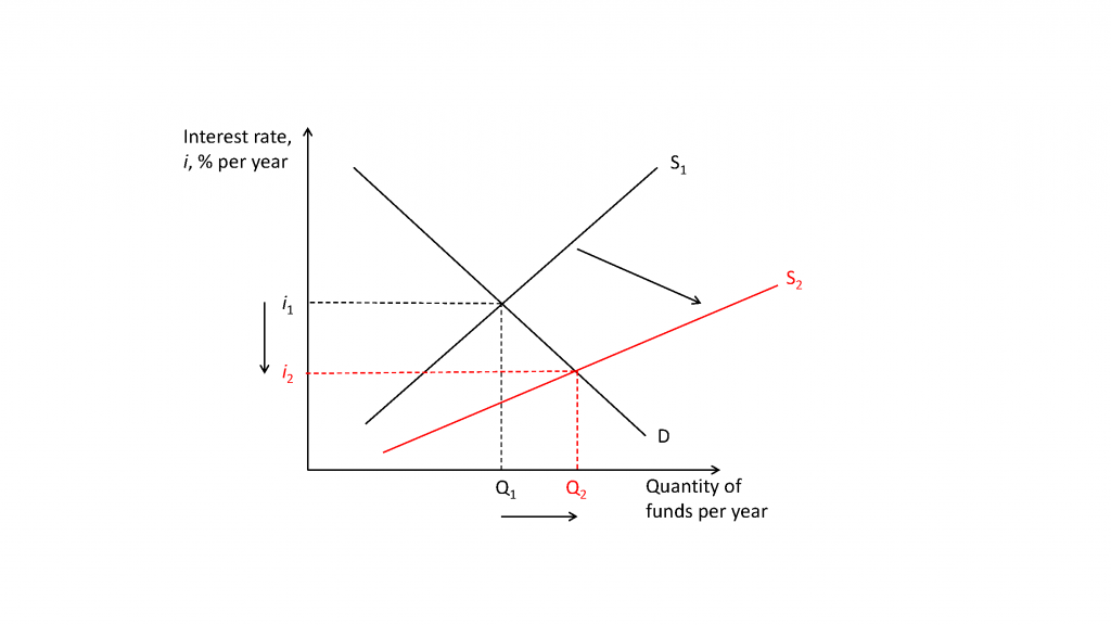
In figure 24.4.1 the capital market it initially in equilibrium at i₁, Q₁. The supply curve represents the amount of funds offered to loan and is upward sloping because as interest rates rise, more funds are made available because of the higher return on loans. The demand curve represents the amount of funds desired to borrow and is downward sloping because as interest rates fall, more funds are desired due to the lower expense of borrowing. At interest rate i₁ the quantity of funds demanded equals the quantity of funds supplied, Q₁. The demand curve will shift based on opportunities to invest, need for funds to pay expenses like to buy a house or pay for college, governments might need money to build roads and buildings, firms might need money to make new investments in plant and equipment, and so on. The supply curve will shift based on things like changes in tax policy that incentivize retirement investment, or due to increased investment among foreigners, or the government policy to buy back government bonds to increase the money supply. In Figure 24.4.1 the supply curve shifts to the right, perhaps due to a new tax policy that incentivizes savings. The effect of the increased supply of funds leads to a lower interest rate, i₂, and a greater amount of funds leant and borrowed, Q₂.

SUMMARY

Review: Topics and Related Learning Outcomes

24.1 Present Discounted Value

Learning Objective 24.1: Explain how money in the future and in the past is given a value in the present.

24.2 Inflation

Learning Objective 24.2: Describe how inflation is accounted for in present value calculations.

24.3 Choices Over Time

Learning Objective 24.3: Describe how individuals can use present value to make decisions over time.

24.4 Interest Rates

Learning Objective 24.4: Explain how interest rates are determined and how they change.

Learn: Key Terms and Graphs

Terms

Interest Rate

Discount Rate

Compounding

Future Value

Present Value

Net Present Value

Capital Market

Graphs

Capital Market Equilibrium

Supplemental Resources