
8
Joel Bruneau and Clinton Mahoney
Learning Objectives
- Explain fixed and variable costs, opportunity cost, sunk cost and depreciation
- Describe the solution to the cost minimization problem in the short-run
- Describe the solution to the cost minimization problem in the long-run
- Analyze the effect of changes in prices or output on total cost
Module 8: Minimizing Costs
The Policy Question: Will an increase in the minimum wage decrease employment?
Recently, a much discussed policy topic in the U. S. is the idea of increasing minimum wages as a response to poverty and growing income inequality. There are many questions of debate about minimum wages as an effective policy tool to tackle these problems, but one common criticism of minimum wages is that they increase unemployment. In this module we will study how firms decide how much of each input to employ in their production of a good or service. This knowledge will allow us to address the question of whether firms are likely to reduce the amount of labour they employ if the minimum wage is increased.
In order to provide goods and services to the marketplace firms use inputs. These inputs are costly, so firms must be smart about how they use labour, capital and other inputs to achieve a certain level of output. The goal of any profit maximizing firm is to produce any level of output at the minimum cost. Doing anything else cannot be a profit maximizing strategy. This module studies the cost minimization problem for firms: how to most efficiently use inputs to produce output.
8.1 The Economic Concept of Cost
Learning Objective 8.1: Explain fixed and variable costs, opportunity cost, sunk cost and depreciation.
8.2 Short-Run Cost Minimization
Learning Objective 8.2: Describe the solution to the cost minimization problem in the short-run.
8.3 Long-Run Cost Minimization
Learning Objective 8.3: Describe the solution to the cost minimization problem in the long-run.
8.4 When Input Costs and Output Change
Learning Objective 8.4: Analyze the effect of changes in prices or output on total cost.
8.1 The Economic Concept of Cost
Learning Objective 8.1: Explain fixed and variable costs, opportunity cost, sunk cost and depreciation.
From the isoquants described in Module 7 we know that firms have many choices of input combinations to produce the same amount of output. Each point on an isoquant represents a different combination of inputs that produces the same amount of output.
Of course inputs are not free: the firm must pay workers for their labour, buy raw materials, and buy or rent machines, all of which are costly. So the key question for firms is: which point on an isoquant is the best choice? The answer is the point that represents the lowest cost. The topics of this module will help us to locate that point.
This module studies production costs; that is, how costs are related to output. In order to draw a cost curve that shows a single cost for each output amount, we have to understand how firms make the decision about which set of possible inputs to use to be as efficient as possible. To be as efficient as possible means that the firm wants to produce output at the lowest possible cost.
For now we assume that firms want to produce as efficiently as possible, in other words, minimize costs. Later, in Module 10: Profit Maximization and Supply, we will see that producing at the lowest cost is what profit maximizing firms must do (otherwise they cannot possibly be maximizing profit!).
A good way to think about the cost side of the firm is to consider a manager who is in charge of running a factory for a large company. She is responsible for producing a specific amount of output at the lowest possible cost. She must choose the mix of inputs the factory will use to achieve the production target. Her task, in other words, is to run her factory as efficiently as possible. She does not want to use any extra inputs and she does not want to pick a mix of inputs that costs more than another mix of inputs that produces the same amount of output.
To make efficient or cost-minimizing decisions it is important to understand some basic cost concepts, starting with fixed and variable costs as well as opportunity costs, sunk costs and depreciation.
Fixed and Variable Costs
A fixed cost is a cost that does not change as output changes. For example a firm might need to pay for the lights to be on in order for the workers to see what they are doing and for production to happen. But the lights are simply on or off and the cost of powering them does not change when output changes.
A variable cost is a cost that changes as output changes. For example a firm that wishes to produce more output might need to employ more labour hours by either hiring more workers or have existing workers work more hours. The cost of this labour is therefore a variable cost as it changes as the output level changes.
Opportunity Costs
As we learned in Module 3, the opportunity cost of something is the value of the next-best alternative given up in order to do get it.
Suppose a firm has access to an input that it can use in production without paying a price for it. A simple example is a family farm. The farm uses land, water, seeds, fertilizer, labour, and farm machinery to produce a crop—let’s say corn–which it then sells in the marketplace. If the farm owns the land it uses to produce the corn, do we then say that the land component is not part of the firm’s costs? The answer, of course, is no. When the farm uses the land to produce corn it forgoes any other use of the land; that is, it gives up the opportunity to use the resource for another purpose. In many cases the opportunity cost is the market value of the input.
For example, suppose an alternative use for the land is to rent it to another farmer. The forgone rent from the decision to use the land to produce its own corn is the farm’s opportunity cost and should be factored in to the production decision. If the opportunity cost, which in this case is the rental fee, is higher than the profit the farm will earn from producing corn, the most efficient economic decision is to rent out the land instead.
Now consider the more complex example of a farm manager who is told to produce a certain amount of corn. Suppose that the manager figures out that she can produce exactly that amount using a low-fertilizer variety of corn and all of the available land. She also knows that another way to produce the same amount of corn is with a higher yielding variety that requires a lot more fertilizer but uses only 75% of the land. The additional fertilizer for this higher yielding corn will cost an extra $50,000. Which option should the farm manager choose?
Without considering the opportunity cost she would use the low-fertilizer variety of corn and all of the land, because it costs $50,000 less than the alternative method. But what if, under the alternative method, she could rent out for $60,000 the 25% of the land that would not be planted? In that case the cost minimizing decision is actually to use the higher yielding corn variety and rent out the unused land.
Another classic example is that of a small business owner who runs, say, a coffee shop. The inputs into the coffee shop are the labour, the coffee, the electricity, the machines and so on. But suppose the owner also works a lot in the shop. He does not pay himself a salary but simply pays himself from the shop’s excess revenues, or revenues in excess of the cost of the other inputs. The cost of his labour for the shop is not $0 but the amount he could earn working elsewhere instead. If, for example, he could work in the local bank for $4,000 a month then the opportunity cost of his working at the coffee shop is $4,000 and if the excess revenues are less than $4,000 he should close the shop and work at the bank instead, assuming he likes both jobs equally well.
Sunk Costs
Some costs are recoverable and some are not. An example of a recoverable cost is the money a farmer spends on a new tractor knowing that she can turn around and re-sell it for the same amount she paid.
A sunk cost is an expenditure that is not recoverable. An example of a sunk cost is the cost of the paint a business owner uses to paint the leased storefront of his coffee shop. Once the paint is on the wall it has no resale value. Many inputs reflect both recoverable and sunk costs. A business that buys a car for the use of an employee for $30,000 and can resell it for $20,000 should consider $10,000 of its expenditure a sunk cost and $20,000 a recoverable cost.
Why do sunk costs matter in choosing inputs? Because after incurring sunk costs, a manager should not consider them in making subsequent decisions. Sunk costs have no bearing on such decisions. To see this, suppose you buy a $500 non-refundable and non-transferrable airline ticket to go to Florida at spring break. However, as spring break approaches you are invited by friends to spend the break at a mountain cabin they have rented to which they will give you a ride in their car at no cost to you. You prefer to spend the break with your friends in the cabin but you have already spent the $500 on the ticket and you feel compelled to get your money’s worth by using it to go to Florida. Doing so would be the wrong decision. At the time of your decision, the $500 spent on the ticket is non-recoverable and therefore a sunk cost. Whether you go to Florida or not you cannot get the $500 back, so you should do what makes you most happy, which is going to the cabin.
Depreciation
Depreciation is the loss of value of a durable good or asset over time. A durable good is a good that has a long usable life. Durable goods are things like vehicles, factory machines or appliances that generally last many years. The difference in the beginning value of a durable good and its value some time later is called depreciation. Most durable goods depreciate: machines wear out, newer more advanced ones are produced reducing the value of current ones, and so on.
Suppose you are a manager who runs a pencil-making factory that uses a large machine. How does -the machine’s depreciation factor into the cost of using it
The appropriate way to think about these costs is through the lens of opportunity cost. If your factory didn’t use the machine you could rent it to another firm, or sell it. Let’s consider the selling of the machine. Suppose it cost $100,000 to purchase the machine new, and it depreciates at a rate of $1,000 per month, meaning that each month its resale value drops by $1,000. Note that the purchase cost of the machine is not sunk because it is recoverable – but each month the recoverable amount diminishes with the rate of depreciation. So, for example, exactly one year after purchase the machine is worth $88,000. At this point in time the $12,000 depreciation has become a sunk cost. However at the current point in time you have a choice: you can sell the machine for $88,000 or use it for a month and sell it at the end of the month for $87,000. The opportunity cost of using the machine for this month is exactly $1,000 in depreciation.
Why does depreciation matter in choosing inputs? Well, suppose workers can do the same job as the machine, or in economics parlance, you can substitute workers for capital. To produce the same amount of pencils as the machine, you need to add labour hours at a rate of $900 a month. A manager without good economics training might think that since the firm purchased the machine the machine is free and since the labour costs $900 a month, use the machine. But you–a manager well trained in economics–know that the monthly cost of using the machine is the $1000 drop in resale value (the depreciation cost) and the monthly cost of the labour is $900. You will save the company $100 a month by using the labour and selling the machine.
8.2 Short-Run Cost Minimization
LO: Describe the solution to the cost minimization problem in the short run.
In order to maximize profits firms must minimize cost. Cost minimization simply implies that firms are maximizing their productivity or using the lowest cost amount of inputs to produce a specific output. In the short run firms have fixed inputs, like capital, giving them less flexibility than in the long run. This lack of flexibility in the choice of inputs tends to result in higher costs.
In Module 7, we studied the short-run production function:
[latex]q=f(L,\overline{K})[/latex]
Where q is output, L is the labour input and K̅ is capital. The bar over K indicates that it is a fixed input. The short-run cost minimization problem is straightforward: since the only adjustable input is labour, the solution to the problem is to employ just enough labour to produce a given level of output.
Figure 8.2.1 illustrates the solution to the short-run cost minimization problem. Since capital is fixed, the decision about labour is to choose the amount which, combined with the available capital, enables the firm to produce the desired level of output given by the isoquant.
Figure 8.2.1: Short-Run Cost Minimization
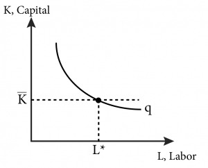
The firm’s short-run cost minimization problem is written as: [latex]min_L[wL+r\overline{K}]\,subject\,to\,q=f(L,\overline{K}),\,where\,\overline{K}\,is\,fixed\,in\,the\,short-run[/latex].
From Figure 8.2.1 it is clear that the only cost minimizing level of the variable input, labour, is at L*. To see this, note that any level of labour below L* would yield a lower level of output, and any level of labour above L* would yield the desired level of output but would be more costly than L* because each additional unit of labour employed must be paid for.
Mathematically this problem requires only that we solve following production function for L:
Solving the production function requires that we invert it, which we can do only if the function is monotonic. This requirement is satisfied for our production functions because we assume that output always increases when inputs increase.
[latex]L*=f^{-1}(\overline{K},q)[/latex]
Let’s consider a specific example of a Cobb-Douglas type production function:
[latex]q=10\overline{K}^{\frac{1}{2}}L^{\frac{1}{2}}[/latex]
To find the cost minimizing level of labour input, L*, we need to solve this equation for L*:
[latex]L^{\frac{1}{2}}=(\frac{q}{10\overline{K}^{\frac{1}{2}}})^2[/latex]
This simplifies to:
[latex]L*=\frac{q^2}{100\overline{K}}[/latex]
Note that this equation does not require a specific output target but rather gives us the cost minimizing level of labour for every level of output. We call this an input demand function: a function that describes the optimal factor input level for every possible level of output.
The minimum cost is then: [latex]C(q)=w\frac{q^2}{100\overline{K}}+r\overline{K},\,where\,\overline{K}\,is\,fixed[/latex].
8.3 Long-Run Cost Minimization
LO: Describe the solution to the cost minimization problem in the long run.
The long run, by definition, is a period of time when all inputs are variable. This gives the firm much more flexibility to adjust inputs to find the optimal mix based on their relative prices and relative marginal productivities. This means that the cost can be made as low as possible, and generally lower than in the short-run.
Total Cost in the Long-Run and the Isocost Line
For a long-run, two-input production function, q=f(L,K), the total cost of production is the sum of the cost of the labour input, L, and the capital input, K.
- The cost of labour is called the wage rate, w.
- The cost of capital is called the rental rate, r.
- The cost of the labour input is the wage rate multiplied by the amount of labour employed: wL.
- The cost of capital is the rental rate multiplied by the amount of capital: rK.
The total cost (C) therefore is:
[latex]C(q)=wL+rK[/latex]
If we hold total cost C(q) constant, we can use this equation to find isocost lines. An isocost line is a graph of every possible combination of inputs that yields the same cost of production. By picking a cost, and given wage rates, w, and rental rates, r, we can find all the combinations of L and K that solve the equation and graph the isocost line.
Consider the example of a pencil making factory where both capital in the form of pencil making machines, and labour to run those machines are utilized. Suppose the wage rate of labour for the pencil maker is $20 per hour and the rental rate of capital is $10 per hour. If the total cost of production is $200 the firm could be employing 10 hours of labour and no capital, 20 hours of capital and no labour, 5 hours of labour and 10 hours of capital or any other combination of capital and labour for which the total cost is $200. Figure 8.3.1 illustrates this particular isocost line.
Figure 8.3.1: An Isocost Line
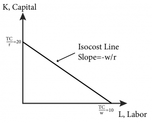
This figure represents the isocost line where total cost equals $200. But we can draw an isocost line that is associated with any total cost level. Notice that any combination of labour hours and capital that is less expensive than this particular isocost line will end up on a lower isocost line. For example 2 hours of labour and 5 hours of capital will cost $90. Any combination of hours of labour and capital that are more expensive than this particular isocost line will end up on a higher isocost line. For example 20 hours of labour and 30 hours of capital will cost $700.
Note that the slope of the isocost line is the ratio of the input prices, –w/r. This tells us how much of one input (capital) we have to give up to get one more unit of the other input (labour) and maintain the same level of total cost. For example if both labour and capital cost $10 an hour, the ratio would be -10/10 or -1. This is intuitive– if they cost the same amount, to get one more hour of labour, you need to give up one hour of capital. In our pencil maker example, labour is $20 per hour and capital is $10 per hour, so the ratio is -2: to get one more hour of labour input you must give up 2 hours of capital in order to maintain the same total cost or remain on the same isocost line.
The solution to the long-run cost minimization problem is illustrated in Figure 8.3.2. The plant manager’s problem is to produce a given level of output at the lowest cost possible. A given level of output corresponds to a particular isoquant so the cost minimization problem is to pick the point on the isoquant that is the lowest cost of production. This is the same as saying the point that places the firm on the lowest isocost line. We can see this by examining Figure 8.3.2 and noting that the point on the isoquant that corresponds to the lowest isocost line is the one where the isocost is tangent to the isoquant.
Figure 8.3.2: The Solution to the Long-Run Cost Minimization Problem
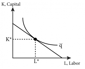
The firm’s long-run cost minimization problem is written as: [latex]min_{LK}[wL+rK]\,subject\,to\,q=f(L,K),\,where\,L\,and\,K\,are\,both\,variable[/latex].
From figure 8.3.2 we can see that the optimal solution to the cost minimization problem is where the isocost and isoquant are tangent: the point at which they have the same slope. We just learned that the slope of the isocost is –w/r and in Module 7 we learned that the slope of the isoquant is the marginal rate of technical substitution (MRTS), which is the ratio of the marginal product of labour and capital:
[latex]MRTS=-\frac{MP_L}{MP_K}[/latex]
So the solution to the long-run cost minimization problem is
[latex]MRTS=-\frac{w}{r}[/latex]
or
[latex]\frac{MP_L}{MP_K}=\frac{W}{T}[/latex]
(8.1)
This can be rearranged to help with intuition:
[latex]\frac{MP_L}{w}=\frac{MP_K}{r}[/latex]
(8.2)
Equation (8.2) says that at the cost minimizing mix of inputs the marginal products per dollar must be equal. This conclusion makes sense if you think about what would happen if Equation (8.2) did not hold. Suppose instead that the marginal product of capital per dollar was more than the marginal product of labour per dollar:
[latex]\frac{MP_L}{w}< \frac{MP_K}{r}[/latex]
This inequality tells us that this current use of labour and capital cannot be an optimal solution to the cost minimization problem. To understand why, consider the effect of taking a dollar spent on labour input away, thereby lowering the amount of labour input (raising the MPL – remember the law of diminishing marginal returns), and spending that dollar instead on capital and increasing the capital input (lowering the MPK). We know from the inequality that if we do this, overall output must increase because the additional output from the extra dollar spent on capital has to be greater than the lost output from the diminished labour. Therefore the net effect is an increase in overall output. The same argument applies if the inequality were reversed.
Calculus Appendix: Long-Run Cost Minimization Problem:
Mathematically we express the long-run cost minimization problem in the following way; we want to minimize total cost subject to an output target.
[latex]\color{green}min_{LK}[wL+rK][/latex]
(8.1C)
[latex]\color{green}subject\,to\,q=\,f(L,K)[/latex]
(8.2C)
We can proceed by defining a Lagrangian function:
[latex]\color{green}\wedge (L,K,\lambda )=wL+rK-\lambda (f(L,K)-q)[/latex]
(8.3C)
where λ is the Lagrange multiplier. The first order conditions for an interior solution (i.e. L > 0 and K > 0) are as follows:
[latex]\color{green}\frac{\partial \wedge}{\partial L}=0\Rightarrow w=\lambda \frac{\partial f(L,K)}{\partial L}[/latex]
(8.4C)
[latex]\color{green}\frac{\partial \wedge }{\partial K}=0\Rightarrow r=\lambda \frac{\partial f(L,K)}{\partial K}[/latex]
(8.5C)
[latex]\color{green}\frac{\partial \wedge }{\partial \lambda }=0\Rightarrow Q=f(L,K)[/latex]
(8.6C)
From module 7 we know that [latex]\color{green}MP_L=\frac{\partial f(L,K)}{\partial L}[/latex] and [latex]\color{green}MP_K=\frac{\partial f(L,K)}{\partial K}[/latex]
[latex]\color{green}\frac{MP_L}{MP_K}=\frac{w}{r}[/latex]
(8.7C)
And 8.6C is the constraint:
[latex]\color{green}q=f(L,K)[/latex]
(8.8C)
8.7C and 8.8C are two equations in two unknowns, L and K, and can be solved by repeated substitution. Note that these are exactly the conditions that describe Figure 8.3.2. 8.7C is the mathematical expression of MRTS = -w/r and 8.8C pins us down to a specific isoquant, as MRTS = -w/r holds for a potentially infinite number of isoquants and isocost lines depending on the q chosen.
An Example of Minimizing Costs in the Long Run
Consider a specific example of a gourmet root beer producer whose labour cost is $20 an hour and whose capital cost is $5 an hour. Suppose the production function for a barrel of root beer, q, is [latex]q=10L^{\frac{1}{2}}K^{\frac{1}{2}}[/latex]. If the output target is 1,000 barrels of root beer, they could, for example, utilize 100 hours of labour, L, and 100 hours of capital, K, to yield 10(10)(10)=1,000 barrels of root beer. But is this the most cost efficient way to do it? More generally, what is the most cost effective mix of labour and capital to produce 1000 barrels of root beer?
To determine this we must start with the marginal products of labour and capital, which for this production function are:
[latex]MP_L=5L^{-\frac{1}{2}}K^{\frac{1}{2}}[/latex]
(8.3)
,
[latex]MP_K=5L^{\frac{1}{2}}K^{-\frac{1}{2}}[/latex]
(8.4)
and
Thus the [latex]MRTS,-\frac{MP_L}{MP_K}\,is:\,-\frac{K}{L}[/latex]
The ratio [latex]-\frac{w}{r}[/latex] in this case is [latex]-\frac{20}{5}[/latex] or -4.
So the condition that characterizes the cost minimizing level of input utilization is:
[latex]\frac{K}{L}=4\, ,or\, K=4\,L[/latex]. That is, for every hour of labour employed, L, the firm should utilize four hours of capital. This makes sense when you think about the fact that labour is four times as expensive as capital. Now what are the specific amounts? To find them we substitute our ratio into the production function set at 1000 barrels:
[latex]1000=10L^{\frac{1}{2}}K^{\frac{1}{2}}[/latex]
(8.5)
If K = 4L then [latex]1000=10L^{\frac{1}{2}}(4L)^{\frac{1}{2}}[/latex] , or [latex]L=\frac{100}{\sqrt{4}}[/latex] which equals 50. If L = 50, then K = 200. So using 50 hours of labour and 200 hours of capital is the most cost effective way to produce 1000 barrels of root beer for this firm.
CALCULUS SUPPLEMENT
- For the following questions the [latex]\color{green} q=5L^{\frac{1}{3}}K^{\frac{2}{3}}[/latex] , w = $30 an hour, r = $15 an hour and the production target q = 1200:
- Find the Marginal Product of Labour.
- Find the Marginal Product of Capital.
- Find the MRTS.
- Find the optimal amount of labour and capital inputs.
- For [latex]\color{green}q=5L^{\frac{1}{3}}K^{\frac{2}{3}}[/latex] and w and r, solve for the input demand functions using the Lagrangian method.
8.4 When Input Costs and Output Change
LO: Analyze the effect of changes in prices or output on total cost.
In the previous section we determined the cost minimizing combination of labour and capital to produce 1,000 barrels of root beer. As long as the prices of labour and capital remain constant, this producer will continue to make the same choice for every 1,000 barrels of root beer produced. But what happens when input prices change?
Suppose, for example, an increasing demand for the capital equipment used to make root beer drives the rental price up to $10 an hour. This means capital is more expensive than before not only in absolute terms but in relative terms as well. In other words, the opportunity cost of capital has increased. Before the price increase, for every extra hour of capital utilized, the root beer firm had to give up ¼ of an hour of labour. After the rental rate increase the opportunity cost has increased to ½ an hour of labour. A cost-minimizing firm should therefore adjust by utilizing less of the relatively more expensive input and more of the relatively less expensive input.
In this case, the ratio [latex]-\frac{w}{r}[/latex] is now [latex]-\frac{20}{10}[/latex] or -2. So the new condition that characterizes the cost minimizing level of input utilization after the price change is:
The production function for 1000 barrels has not changed:
[latex]1,000=10L^{\frac{1}{2}}K^{\frac{1}{2}}[/latex]
So, if K = 2L then [latex]1000=10L^{\frac{1}{2}}(2L)^{\frac{1}{2}}[/latex], or [latex]L=\frac{100}{\sqrt{2}}[/latex] which equals roughly 71. If L = 71, then K = 2L = 142. As expected the firm now uses more labour than it did prior to the price change and less capital.
We can also calculate and compare the total cost before and after the increase in the rental rate for capital. Total cost is C(q) = wL + rK. So in the first case where w is $20 and r is $5 the total cost is:
C(q) = 20(L) + 5(K) = $20(50) + $5(200) = $1000 + $1000 = $2000
Now, when capital rental rates increase to $10, total cost becomes:
C(q) = 20(L) + 10(K) = $20(71) + $10(142) = $1420 + $1420 = $2840
This new higher cost makes sense because the production function did not change so the firm’s efficiency remained constant, wages remained constant but rental rates increased. So overall the firm saw a cost increase and no change in productivity leading to an increase in production costs.
Expansion Path
A firm’s expansion path is a curve that shows the cost-minimizing amount of each input for every level of output. Let’s look at an example to see how the expansion path is derived.
Equation 8.5 describes the production function set to the specific production target of 1000 barrels of root beer. If we replace 1000 with the any output level q, we get the following expression:
We use the K = 4L ratio of capital to labour that characterizes the cost minimizing ratio when the wage rate for labour is $20 an hour and the rental rate for capital is $5 an hour:
- If [latex]K=4L,\,then\,q=10L^{\frac{1}{2}}(4L)^{\frac{1}{2}}\, ,or\,q=20L\,or\,L(q)={\frac{q}{20}}[/latex].
- If [latex]L(q)=\frac{q}{20'}\,then\,K(q)=\frac{4q}{20}=\frac{q}{5}[/latex].
So using 50 hours of labour and 200 hours of capital is the most cost effective way to produce 1,000 barrels of root beer for this firm.
Note that [latex]L(q)=\frac{q}{20}[/latex] and [latex]K(q)=\frac{4q}{20}=\frac{q}{5}[/latex] are both functions of output, q. These are the input demand functions.
Input demand functions describe the optimal, or cost-minimizing, amount of a specific production input for every level of output. Note that when the output q = 1,000, L(q) = 50 and K(q) = 200 just as we found before. But from these factor demands we can immediately find the optimal amount of labour and capital for any output target at the given input prices. For example, suppose the factory wanted to increase output to 2000 or 3000 barrels of root beer:
At [latex]q=2,000, L(2000)=\frac{2000}{20}=100\,and\,K(2000)=\frac{2000}{5}=400[/latex]
We can graph this firm’s expansion path (Figure 8.4.1) from the input demands when q equals 1,000, 2,000 and 3,000. We can also immediately derive the long run total cost curve from these factor demands by putting them into the long run cost function, [latex]C(q)=wL+rK[/latex] :
[latex]C(q)=wL+rK=wL(q)+rK(q)=w\frac{q}{20}+r\frac{q}{5}[/latex]
At input prices w = $20 and r = $5, the function becomes [latex]C(q)=20\frac{q}{20}+5\frac{q}{5}=2q[/latex]
The long-run total cost curve shows us the specific total cost for each output amount when the firm is minimizing input costs.
Graphically, the expansion path and associated long-run total cost curve look like Figure 8.4.1.
Figure 8.4.1: The Expansion Path and Long-Run Cost Curve
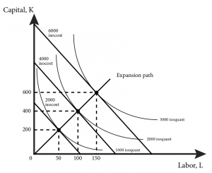
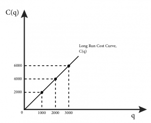
Figure 8.4.1 illustrates how the solution to the cost minimization problem translates into factor demands and long-run total cost. We can solve for the factor demands and the total cost function more generally by replacing our specific input prices with w and r in the following way. The solution to the cost minimization problem is characterized by the MRTS equaling the input price ratio:
[latex]q=10L^{\frac{1}{2}}K^{\frac{1}{2}}=10(\frac{rK}{w})^{\frac{1}{2}}\,K^{\frac{1}{2}}=10(\frac{r}{w})^{\frac{1}{2}}\,K[/latex]
Solving for the input demand for capital yields:
Since [latex]L=\frac{rK}{w}[/latex] we can find the input demand for labour:
[latex]L*=\frac{q}{10}(\frac{r}{w})^{\frac{1}{2}}[/latex]
Now we have input demand functions that are functions of both output, q, and the input prices, w and r. Note that when q rises, the inputs of both capital and labour rise as well. Also note that when the price of labour, w, rises relative to the price of capital, r, or when [latex]\frac{w}{r}[/latex] rises, the use of the capital input rises and the use of the labour input falls. And when the price of capital rises relative to the price of labour, the use of labour rises and the use of capital falls. So from these functions we can see the firm’s optimal adjustment to changing input costs in the form of substituting the relatively cheaper input for the relatively more expensive input.
Perfect Complement and Perfect Substitute Production Functions
Perfects complements and perfect substitutes in production are not uncommon. Consider if our pencil making firm that needs exactly one operator (labour) to operate one pencil making machine. A second worker per machine adds nothing to output and a second machine per worker also adds nothing to output. In this case the pencil making firm would have a perfect complements production function. Alternatively, suppose our root beer producer could use either two workers (labour) to measure and mix up the ingredients or could employ one machine to do the same job. Either combination yields the same output. In this case the root beer producer would have a perfect substitutes production function.
Similar to the consumer choice problem, for production functions where inputs are perfect complements or substitutes the condition MRTS equals the price ratio will no longer hold. To see this, consider figure 8.4.2.
Figure 8.4.2: The Long-Run Cost Minimization Solution for Perfect Complements (a) and Perfect Substitutes (b, c)
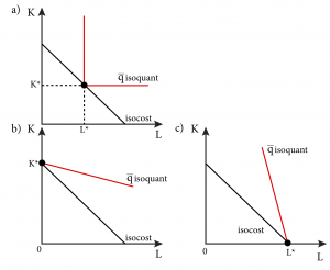
In panel (a), a perfect complements isoquant just intersects the isocost line at the corner of the isoquant. (Take a moment and confirm to yourself that any other combination of labour and capital on the isoquant would be more expensive.) However, at the corner of the isoquant the slope is undefined, so there is no MRTS. For perfect complements, using inputs in any combination other than the optimal ratio is not cost minimizing. So we can immediately express the optimal ratio as a condition of cost. If the production function is of the perfect complement type, [latex]q=min[\alpha L,\beta K][/latex], the optimal input ratio is
Panels (b) and (c) of Figure 8.4.2 show the optimal solution to the long-run cost minimization problem when the production function is a perfect substitutes type. The solution is on one corner or the other of the isocost line, depending on the marginal productivities of the inputs and their costs. In (b), the MRTS or the slope of the isoqant is lower (less steep) than the slope of the isocost line or the ratio of the input prices. Since this is the case it is much less costly to employ only capital to produce q. In (c), the MRTS or the slope of the isoqant is higher (more steep) than the slope of the isocost line or the ratio of the input prices. Since this is the case it is much less costly to employ only labour to produce q.
Recall that a perfect substitutes production function is of the additive type:
[latex]q=\alpha L+\beta K[/latex]
The marginal product of labour is α and the marginal product of capital is β.
Since the MRTS is the ratio of the marginal products, the MRTS is [latex]\frac{\alpha}{\beta}[/latex], which is also the slope of the isoquant.
The ratio of input prices is [latex]\frac{w}{r}[/latex]. This price ratio is the slope of the isocost.
From the graphs we can see that if [latex]\frac{\alpha }{\beta }< \frac{w}{r}[/latex], or the isoquant is less steep than the isocost, only capital is used, thus we know that no labour will be employed, or L *= 0 , and output must equal [latex]\beta K\,or\,q=\beta K[/latex]. Solving this for K gives us: [latex]K*=\frac{q}{\beta}[/latex]. Alternatively, if [latex]\frac{\alpha }{\beta }> \frac{w}{r}[/latex], only labour is used, so [latex]K*=0\, ,\,q=\alpha L\, ,\, and \,L*=\frac{q}{\alpha}[/latex].
SUMMARY
Review: Topics and Related Learning Outcomes
8.1 The Economic Concept of Cost
Learning Objective 8.1: Explain fixed and variable costs, opportunity cost, sunk cost and depreciation.
8.2 Short-Run Cost Minimization
Learning Objective 8.2: Describe the solution to the cost minimization problem in the short-run.
8.3 Long-Run Cost Minimization
Learning Objective 8.3: Describe the solution to the cost minimization problem in the long-run.
8.4 When Input Costs and Output Change
Learning Objective 8.4: Analyze the effect of changes in prices or output on total cost.
Learn: Key Terms and Graphs
Terms
Graphs
The Solution to the Long-Run Cost Minimization Problem
The Expansion Path and Long-Run Cost Curve
The Long-Run Cost Minimization Solution for Perfect Complements and Perfect Substitutes
Equations
Supplemental Resources
Practice Questions
YouTube Videos
These videos from the YouTube channel ‘Department of Economics’ may be helpful.
- Intermediate Microeconomics: Cost Minimization, Part 1 – YouTube
- Intermediate Microeconomics: Cost Minimization, Part 2 – YouTube
- Intermediate Microeconomics: Expansion Paths – YouTube
- Intermediate Microeconomics: Short Run Type 1 Summary – YouTube
- Intermediate Microeconomics: Short Run Cost Function: Introduction – YouTube
- Intermediate Microeconomics: Short Run Total Costs: Type 1 – YouTube
- Intermediate Microeconomics: Short Run Average and Marginal Costs: Type 1 – YouTube
- Intermediate Microeconomics: Short Run Total Costs, Type 2 – YouTube
- Intermediate Microeconomics: Short Run Average and Marginal Costs, Type 2 – YouTube
- Intermediate Microeconomics: Short Run to Long Run, Part 1 – YouTube
- Intermediate Microeconomics: Short Run to Long Run, Part 2 – YouTube
- Intermediate Microeconomics: Short Run to Long Run, No Crossing – YouTube
- Intermediate Microeconomics: Short Run to Long Run, Conclusion – YouTube
- Intermediate Microeconomics: Long Run Total Cost – YouTube
Policy Example
Policy Example: Will an Increase in the Minimum Wage Decrease Employment
Learning Objective: Apply the concept of cost minimization to a minimum wage policy.
On May 15, 2014 the city of Seattle, Washington passed an ordinance that established a minimum wage of $15 an hour, almost $5 more than the statewide minimum wage and more than double the federal minimum of $7.25 an hour. [http://murray.seattle.gov/minimumwage/#sthash.DOMR7lEp.dpbs]
A minimum wage raises many issues about its impact, particularly for a city surrounded by suburbs that allow much lower rates of pay. One question we can answer with our current tools is how Seattle-based businesses affected by the increased minimum wage are likely to react to the higher cost of labour.
Most businesses that employ labour have many other inputs as well, some of which can be substituted for labour. Consider a janitorial firm that sells floor cleaning services to office buildings, restaurants, and industrial plants. The janitorial firm can choose to clean floors using a small amount of capital and a large amount of labour: they can employ many cleaners and equip them with a simple mop.

Or they could choose to employ more capital in the form of a modern floor-cleaning machine and employ fewer cleaners.
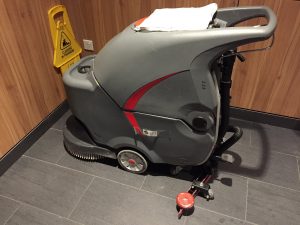
Our theory of cost minimization can help us understand and predict the consequences of making the labour input for cleaning the floors 50% more expensive. Figure 1 shows a typical firm’s long-run cost minimization problem. It is reasonable to consider the long-run in this case because it would not take the firm very long to lease or purchase and have delivered a floor cleaning machine. It is also reasonable to assume that floor cleaning machines and workers are substitutes but not perfect ones – meaning that machines can be used to replace some labour hours, but some machine operators are still needed. The opposite is also true: the restaurant can replace machines with labour but labour needs some capital (a simple mop) to clean a floor.
Figure 1: Change in Inputs Due to Increase in Wages
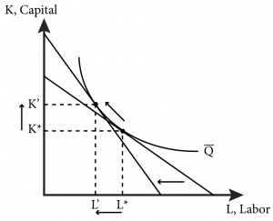
In Figure 1 the isoquant, [latex]\overline{Q}[/latex], represents the fixed amount of floor the firm needs to clean each day and the different combinations of capital and labour it can use to achieve that output target. When the cost of labour, w, increases and the cost of capital, r, stays the same, the isocost line gets steeper as w/r increases. We can see in the figure that when this happens the firm will naturally shift away from using the relatively more expensive input and toward the relatively cheaper input. The restaurant will decrease the amount of labour it employs and increase the amount of capital it uses.
From this specific firm, we can generalize that a dramatic permanent increase in the minimum wage will cause affected firms to employ fewer hours of labour, and that employment overall will fall in the affected area. The magnitude of employment change caused by such a policy depends on the production technology of all affected firms–that is, how easy it is for them to substitute more capital. All we can predict with our model currently is the fact that such shifts away from labour will likely occur. Whether the cost of this decrease in employment is outweighed by the benefit of such a policy is beyond the scope of the current analysis, but our model of cost minimization has provided useful insight into the decisions firms will make in reaction to the increase in minimum wage.
Exploring the Policy Question
- Do you support a national minimum wage increase? Why or why not?
- Do you think the benefits of a minimum wage increase outweigh the costs? Explain your answer.
- What do you predict would happen if, instead of a minimum wage, a tax on the purchase or rental of capital equipment was imposed?
Candela Citations
- Authored by: Joel Bruneau & Clinton Mahoney. License: CC BY-NC-SA: Attribution-NonCommercial-ShareAlike
- Module 7: Minimizing Costs. Authored by: Patrick Emerson. Retrieved from: https://open.oregonstate.education/intermediatemicroeconomics/chapter/module-7/. License: CC BY-NC-SA: Attribution-NonCommercial-ShareAlike
- Input Demand. Authored by: Preston McAfee & Tracy R Lewis. Retrieved from: https://resources.saylor.org/wwwresources/archived/site/textbooks/Introduction%20to%20Economic%20Analysis.pdf. License: CC BY-NC-SA: Attribution-NonCommercial-ShareAlike
of production is the cost of production that does not vary with output level; the fixed cost is the cost of the fixed inputs in production, such as the cost of a machine (capital) that costs the same to operate no matter how much production is happening
of production is the cost of production that varies with output level. This is the cost of the variable inputs in production, for example the cost of the workers that assemble the electronic devices along a conveyor belt
the opportunity cost of something is the value of the next-best alternative given up in order to do get it
is an expenditure that is not recoverable
is the loss of value of a durable good or asset over time
is a good that has a long usable life
is a period of time in which some inputs are fixed
this input category describes all of the machines that are used in production, such as conveyor belts, robots, and computers. It also describes the buildings, such as factories, stores, and offices, and other non-human elements of production, such as delivery trucks
is a period of time long enough that all inputs can be adjusted
a curve that shows all of the possible combinations of inputs that produce the same output
a mathematical expression of the maximum output that results from a specific amount of each input
is a function that describes the optimal factor input level for every possible level of output
is a graph of every possible combination of inputs that yields the same cost of production
is a curve that shows the cost-minimizing amount of each input for every level of output
