
14
Joel Bruneau and Clinton Mahoney
Learning Objectives
- Explain the conditions that lead to monopolies
- Explain how monopolists maximize profits and solve for the optimal monopolist’s solution from a demand curve and a marginal cost curve
- Describe the relationship between demand elasticity and a monopolist’s ability to price above marginal cost
- Describe the how monopolists create deadweight loss and explain how deadweight loss affects societal welfare
Module 14: Monopoly
Policy Example: Should the Government Give Patent Protection to Companies That Make Live-Saving Drugs?
In 1993 Shionogi, a Japanese pharmaceutical company received a patent for the anti-statin medication rosuvastatin calcium, better known by its brand name: Crestor. Crestor is used to treat high-cholesterol and related heart and cardiovascular disease. Crestor has become one of the best selling drugs of all time. In 2016, the patent protection will expire and AstraZeneca, the manufacturer of Crestor, will cease to be a monopolist in the market for Crestor as generic versions of the drug will flood the market place. The patent created a 23-year monopoly in the Crestor market for which it has enjoyed enormous profits; Astra Zeneca recorded $5 billion in Crestor sales in 2015 alone.
Providing a company the exclusive rights to sell a popular and medically important drug creates the potential for enormous profits, which gives pharmaceutical companies a very strong incentive to invest in the research and development of new drugs. But it also creates a situation in which medically necessary drugs are very expensive for consumers.
Exploring the Policy Question
- Does the societal benefit from the advent of new drugs outweigh the cost to society from the creation of monopolies?
- What other way could society promote the development of new medicines?
14.1 Conditions for Monopoly
Learning Objective 14.1: Explain the conditions that lead to monopolies.
14.2 Profit Maximization for Monopolists
Learning Objective 14.2: Explain how monopolists maximize profits and solve for the optimal monopolist’s solution from a demand curve and a marginal cost curve.
14.3 Market Power and the Demand Curve
Learning Objective 14.3: Describe the relationship between demand elasticity and a monopolist’s ability to price above marginal cost.
14.4 Monopoly and Welfare
Learning Objective 14.4: Describe the how monopolists create deadweight loss and explain how deadweight loss affects societal welfare.
14.1 Conditions for Monopoly
Learning Objective 14.1: Explain the conditions that lead to monopolies.
A Monopoly is the sole supplier of a good for which there does not exist a close substitute. In the policy example above a firm that make the only drug with which to treat or cure a disease is a monopolist if there is no other drug available to treat or cure the disease or if the only other drugs are not nearly as effective. Many drug makers continue to hold onto their trademarked drug names even after the patents run out and generic drugs enter the market, but the presence of the generics means that the original companies are no longer monopolists in the market for that particular drug.
As we learned in Module 13, the characteristics of monopoly markets are a single firm, a unique product and barriers to entry. But what are those barriers to entry and where to they come from? There are two main sources of these barriers: cost conditions that make it cheaper for one firm to produce than for many and government regulations that create legal barriers to entry that prevent other firms from competing in the same market.
Cost Advantages can come from a number of sources. A firm might control an essential input, for example one company might control the only source of a rare earth element use in high performance batteries for automobiles. A firm might have a better technology or method of producing a good or service that gives it a cost advantage. Of course this advantage only lasts as long as the firm is the only one with the technology or method. For this reason, many firms keep their production processes a closely guarded secret.
Another source of monopoly are very large fixed costs associated with production. If the fixed costs of production are large enough relative to the demand for a product, it may be true that only one firm can make non-negative economic profits. This is referred to as a natural monopoly: when one firm can supply the market more cheaply than two or more firms. For example suppose an entrepreneur wants to start a concrete pumping service in her isolated small town to provide poured concrete to difficult to reach places that normal concrete trucks are unable to pull up to. Concrete pumping trucks are very large and very expensive. The town might have enough demand to justify the cost of one such truck, the entrepreneur will attract enough business to cover the cost of the truck itself and the other accounting and opportunity costs of the business. But there might not be enough demand to justify the purchase of a second concrete pumping truck if another business decided to start up. Thus the monopoly that results is a natural result of the large fixed cost relative to the limited demand.
We can express the concrete pumping example more formally with a simple model. Suppose the marginal cost of supping pumped concrete is fixed at c and the cost of the truck itself, the fixed cost, is F. The truck is a fixed cost because it costs F to acquire the truck and this does not depend on the amount of concrete sold, Q. The firms total cost function is therefore: TC = cQ + F. Average cost is: AC = c + F/Q. This is the same for any firm that enters the market. Let’s say that the cost of the truck, F, annualized, is $500,000 per year and the marginal cost is $1 per cubic foot of concrete, Q. Now suppose that the demand is such that at MC = $1, 100,000 cubic feet of concrete is sold per year. If there is one firm the average cost of pumped concrete is AC = $1 + $500,000/100,000. Or AC = $6. If there were two firms the average cost of the industry would be ACIND = c + 2F/Q. Note that at a constant MC, the cost of a single cubic foot of concrete is always c no matter which company provides it, however, with two firms there are two fixed costs because each one has to pay for a truck. So AC = $1 + $1,000,000/100,000, or AC = $11. If the maximum willing ness to pay for concrete at 100,000 cubit feet a year in this town is $8, the town can only support one firm. One firm would make $2 in economic profit in this business while two firms would each lose $3 in economic profit.
Another important source of monopoly power is government. The government itself owns and manages monopolies, for example the federal government runs the U.S. Postal Service, and local governments are often the sole provider of utilities such as water and sewer services. The government also provides protection from competition for individual firms, guaranteeing their monopoly status. The most common protection the government offers is patent protection but government can also require licenses to operate businesses, for example to a local hospital, and issue only one per market or they can grant a firm the right to operate as a monopoly, for example a municipality might grant one company the right to collect residential trash.
A patent is an exclusive right to an invention, which excludes others from making, using, selling or importing it into the country for a limited time. In other words, the inventor is granted protection from any direct competition for a time period, generally 20 years form the time an application is filed, and in exchange the invention becomes public knowledge when the patent is granted. Why does the government offer patent protection? As we will see in the next section, being a monopolist often allows companies to collect positive economic profits – a better than normal return on investment. So patents give companies a reward for investing in new technologies, new drugs and new methods that are valuable to society in order to incentivize them into investing in such discoveries.
14.2 Profit Maximization for Monopolists
Learning Objective 14.2: Explain how monopolists maximize profits and solve for the optimal monopolist’s solution from a demand curve and a marginal cost curve.
All profit maximizing firms, regardless of the structure of the markets in which they sell, maximize profits by setting output such that marginal revenue equals marginal cost as we learned in Module 10. Module 9 demonstrated how to find a marginal cost curve from the firm’s total cost curve. What is different in the case of monopoly is the marginal revenue curve. Perfectly competitive firms take prices as given, their output decisions do not change market prices and so the marginal revenue for a perfectly competitive firm is simply the market price. Monopolists, on the other hand, are ‘price makers’ in the sense that they can set their prices by picking a point on the demand curve. Note that they are not free of constraint; the demand curve dictates the maximum price they can charge for every quantity level. The task for the profit-maximizing monopolist is to determine which point on the demand curve maximizes their profits. A downward sloping demand curve will mean that the firm faces a trade-off: they can sell more but must lower their price to do so. This means that the marginal revenue of a monopolist will depend on their output decision.
The total revenue for a firm is the amount of goods they sell, Q, multiplied by the price at which they sell the goods, p. Note that Q is both the firm’s output and the market output as there is only the one firm supplying the market.
TR = pQ
The firm’s marginal revenue is the change in total revenue from the sale of one more unit of their output. Thus a firm that earns ∆TR extra revenue from the sale of ∆Q more units has a marginal revenue of:
[latex]MR=\frac{∆TR}{∆Q}[/latex]
Therefore if the firm sells one more unit, ∆Q=1, and MR=∆TR
Calculus note: Marginal revenue can be found from total revenue by taking the derivative:
Because of the price-quantity trade off from the demand curve, the marginal revenue of a monopolist will depend on its output. Unlike a perfectly competitive firm whose product sells for a constant price and therefore its marginal revenue is that constant price, a monopolist who wants to sell one more unit must lower its price to do so. Thus a monopolist’s marginal revenue is a constantly declining function. It also declines at a rate greater than the demand curve because to sell more the monopolist must lower the price of all its goods. Figure 14.2.1 demonstrates the marginal revenue trade off.
Figure 14.2.1: Monopoly, Revenue and Marginal Revenue
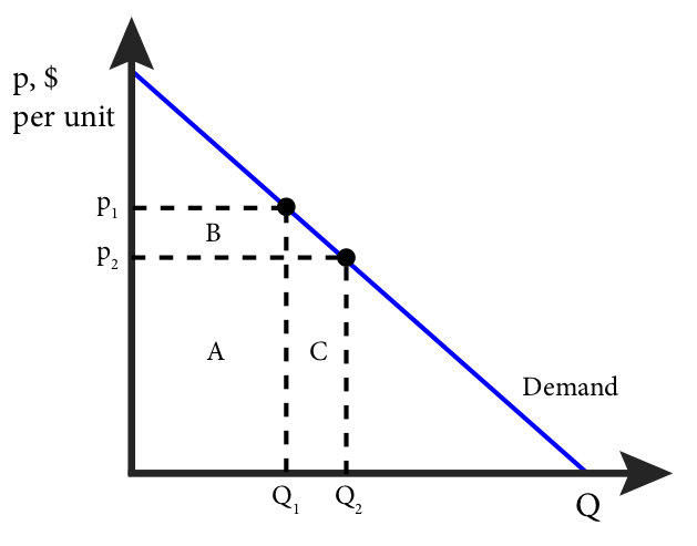
At price p1 the total revenue is p1Q1, which is represented by the areas A+B. At price p2 the total revenue is p2Q2, which is represented by the areas A+C. Area A is the same for both so the marginal revenue is the difference between B and C or C-B.
Note that area C is the price, p2, times the change in quantity, Q2 – Q1, or p∆Q; and area B is the quantity, Q1, times the change in price, p2 – p1, or ∆pQ. Since p2 – p1 is negative, the change in total revenue is C-B or:
Dividing both sides by ∆Q gives us an expression for marginal revenue:
(14.1)
This expression has an intuitive interpretation. The first part, p, is the extra revenue the firm gets from selling an extra unit of the good. The second part,[latex]Q\frac{\Delta p}{\Delta Q}[/latex] , which is negative, is the decrease in revenue from the fact that increasing output marginally, lowers the price the firm receives for all of its output. Since the second part is negative we know that the MR curve is below the demand curve for every Q since demand curve relates price and quantity.
Figure 14.2.2 shows the relationship between a linear demand curve and the marginal revenue curve in the top panel and the total revenue in the bottom panel.
Figure 14.2.2: Demand, Marginal Revenue and Total Revenue
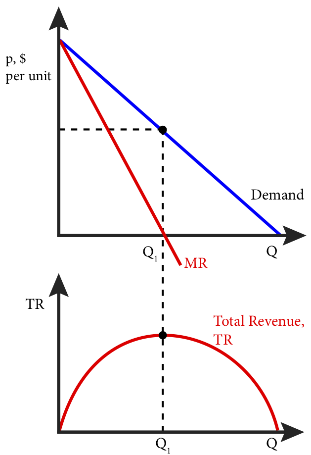
Since marginal revenue is the rate of change in total revenue for a marginal increase in quantity, when marginal revenue is positive, the total revenue curve has a positive slope, and when marginal revenue is negative, the total revenue curve has a negative slope. Note that this means the total revenue is maximized at the point where marginal revenue is zero.
A profit maximizing firm chooses output such that the marginal cost of producing that output exactly matches the marginal revenue it gets from selling that output. Now that we have the marginal revenue all that remains is to add the marginal cost. Figure 14.2.3 shows the optimal output for the monopolist where marginal revenue and marginal cost intersect.
Figure 14.2.3: Profit Maximization for a Monopolist
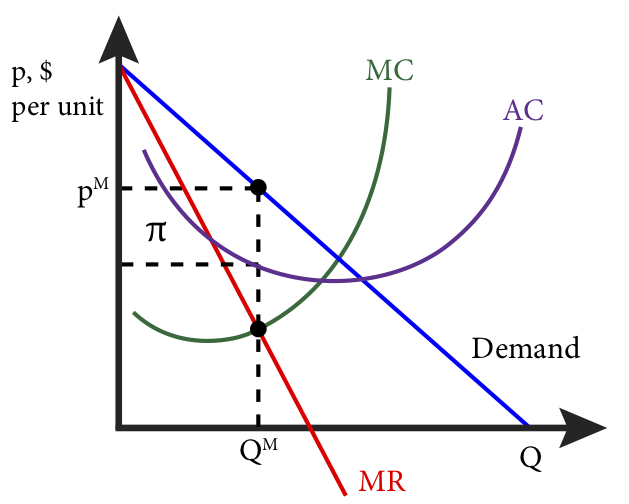
The intersection of the marginal revenue and marginal cost curves occurs at point QM and the highest price at which the monopolist can sell exactly QM is pM. At QM the total revenue is simply (pM) × (QM), and total cost is (AC) × (QM) since AC is just TC/Q. Therefore the shaded area is the difference between total revenue and total cost or profit.
Mathematically, profit maximization for a monopolist is the same as for any firm: find the output level for which marginal revenue equals marginal cost. Let’s start with a general example. Suppose the demand for a good produced by a monopolist is p = A – BQ. Note that this is an inverse demand curve a demand curve written with price as a function of quantity. We could easily solve it for Q to get it back in normal form: Q = A/B – p/B. We can find the marginal revenue curve by first noting that TR = p × Q. Thus TR = (A – BQ) × Q, or TR = AQ – BQ2.
Calculus component:
If TR = AQ – BQ2, then
The marginal revenue from a linear demand curve is a curve with the same vertical intercept as the demand curve, in this case A, and a slope twice as steep, in this case -2B. In other words, for an inverse demand curve, p = A – BQ, the marginal revenue curve is MR = A – 2BQ.
Let’s consider a specific example. Suppose that Tesla is a monopolist in the manufacture of luxury electric cars and faces an annual demand cure for its electric Model S cars of Q = 200 – 2p (in thousands). It has a marginal cost of producing a Model S of MC = Q (also in thousands).
First, we will solve for the monopolist’s profit maximizing level of output and the profit maximizing monopolist’s price. Second, we will graph the solution.
To solve the problem we need to proceed in four steps: one, find the inverse demand curve; two, find the marginal revenue curve; three, set marginal revenue equal to marginal cost and solve for QM, the monopolist’s profit maximizing output level; four, find pM the monopolist’s profit maximizing price.
1) We find the inverse demand curve by solving for demand curve for p:
Q = 200 – 2p
2p = 200 – Q
p = 100 – ½ Q
2) We find the marginal revenue curve by doubling the slope coefficient (B):
MR = 100 – (2)×(½) Q
MR = 100 – Q
3) Set MR equal to MC and solve for Q:
MR = MC
100 – Q = Q
100 = 2Q
QM = 50
or
QM = 50,000
4) Find pM from the inverse demand curve:
p = 100 – ½ Q
p = 100 – ½ (50)
p = 100 – 25
pM = $75
or
pM = $75,000
So the optimal output of Model S cars for Tesla is 50,000 cars and the optimal price is $75,000 per car.
Figure 14.2.4: Solution to Tesla’s Profit Maximization Problem
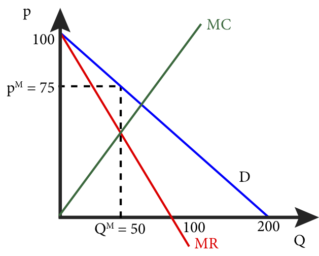
In order to determine Tesla’s profit, we need the total cost function. Suppose total cost is TC = ½ Q2. In this case, with a QM = 50 and pM = $75, the total revenue, TR = $75 × 50 = $3750, or $3.75 million. Total cost is TC = ½ (50)2 = $1250 or $1.25 million. So profit, which is TR – TC, equals $2500 or $2.5 million.
14.3 Market Power and the Demand Curve
Learning Objective 14.3: Describe the relationship between demand elasticity and a monopolist’s ability to price above marginal cost.
A firm that faces a downward sloping demand curve has market power: the ability to choose a price above marginal cost. Monopolists face downward sloping demand curves because they are the only supplier of a particular good or service and the market demand curve is therefore the monopolist’s demand curve. How much market power a firm has is a function of the shape of the demand curve. A market in which customers are very price sensitive is one with a highly elastic demand curve or one that is relatively flat. A market in which customers are very price insensitive is one with a highly inelastic demand curve or one that is relatively steep. What makes customers more or less price sensitive? A number of factors but the most important one is the availability of good substitutes. A drug company who has a patent for a drug that is the only cure for a serious disease is likely to face an inelastic demand curve as those that have the disease will be likely to buy at any price they can afford since there is no other choice. However, a smart-phone company that has a patent for its unique technologies would probably face a highly elastic demand curve because customers would be likely to switch to a different smart-phone with slightly different capabilities if the price was too much higher.
Consider Tesla, the example from 14.2: Tesla arguably has a monopoly on luxury all-electric cars. But there are may other non-luxury all electric cars and luxury hybrid cars with both gas and electric motors. Tesla’s demand curve is probably somewhere in between the two examples above. There are substitutes but they are quite a bit different from the Tesla and so customers of Tesla are probably fairly price insensitive.
The relationship between the elasticity of the demand curve that a monopolist faces and the monopolist’s ability to price above its marginal cost can be derived by using the marginal revenue equation (14.1):
[latex]MR=p+Q\frac{∆p}{∆Q}[/latex]
Profit maximization implies that MR = MC so:
[latex]p+Q\frac{∆p}{∆Q}=MC[/latex]
If we multiply [latex]Q\frac{\Delta p}{\Delta Q}[/latex]by [latex]\frac{p}{p}[/latex]we don’t change the value since
[latex]p+(\frac{Δp}{Δq}x\frac{Q}{p})xp=MC[/latex]
Notice that the term in the parentheses is the inverse of the elasticity,[latex]\frac{1}{\varepsilon}[/latex], from Module 5 so:
[latex]p+(\frac{1}{ε})×p=MC[/latex]
Rearranging terms yields:
(14.2)
We call the left-hand side of this equation the markup: the percentage amount the price is above marginal cost. The right hand side of the equation says that the markup is inversely related to the elasticity of the demand. As consumers are more price sensitive, the absolute value of the elasticity increases causing the right-hand side of the equation to decrease, meaning the markup decreases – monopolists are not able to charge as high a price as if they faced price-insensitive customers. This equation (14.2) has a special name, it is called the Lerner Index, and it measures the firm’s optimal markup. This is also a measure of market power as firms with more market power are more able to change prices above marginal cost. Notice that when the demand curve is perfectly elastic, or horizontal, the monopolist is in the same situation that a perfectly competitive firm is. Perfect elasticity implies that ε=-∞ or that the right-hand side of the Lerner Index is essentially zero meaning the monopolist sets price equal to marginal cost just as if they were a perfectly competitive firm. On the other extreme, a perfectly inelastic demand curve has an elasticity of close to zero. In this case, the markup is infinitely high.
We know from figure 14.2.2 that a monopolist firm will never want to operate on the inelastic part of the demand curve and the Lerner Index confirms that if [latex]\left | e \right |< 1[/latex],the index is greater than one and this implies that p-MC > p which can only be true if marginal cost is negative and marginal cost never negative.
The relationship between markup and demand elasticity can be seen graphically as in Figure 14.3.1.
Figure 14.3.1: Markup and the Shape of the Demand Curve
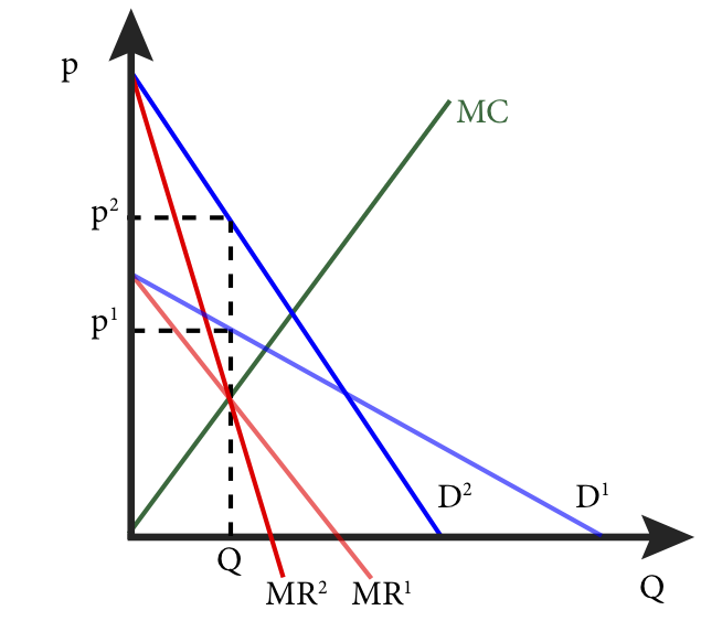
In the figure above, D1 is demand curve that is much more elastic than D2. This means that if the monopolist tries to charge higher prices it loses more sales than if it faced D2. This constrains the monopolist and therefore p1 is significantly lower than p2. As an example using the Lerner Index, suppose at Q the elasticity from D1 is -4 and the elasticity from D2 is -2. The Lerner Index for p1 is ¼ or .25 or a 25% markup. The Lerner Index for p2 is ½ or .5 or a 50% markup.
14.4 Monopoly and Welfare
Learning Objective 14.4: Describe the how monopolists create deadweight loss and explain how deadweight loss affects societal welfare.
In Module 11 we learned that welfare is defined as the sum of consumer and producer surplus. Perfectly competitive markets that meet a set of criteria maximize welfare and achieve efficiency. Monopoly markets do not. To understand why not, think about the marginal revenue relationship to the demand curve as explained in 14.2. The monopolist’s incentive is to limit output in order to keep prices high for all of its goods.
Figure 14.4.1: Monopoly and Deadweight Loss
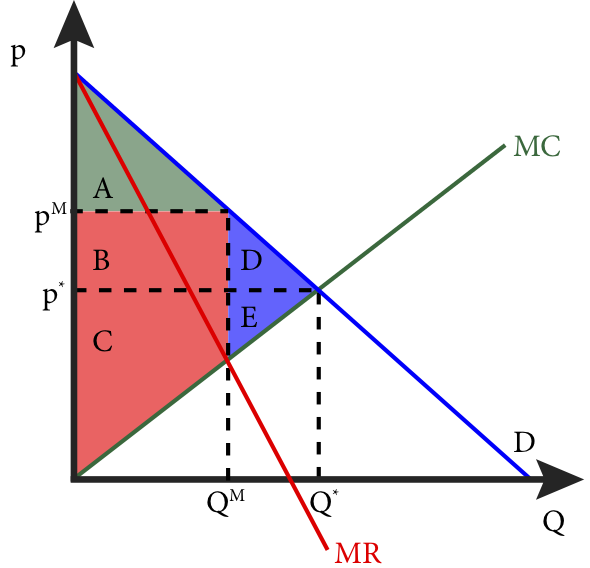
In Figure 14.4.1 the monopolist output, QM, and the monopolist’s price, pM, create an area of consumer surplus of A. The producer surplus is area B+C and the total surplus is A+B+C. We can compare this outcome to the perfectly competitive outcome which is shown as p* and Q*, or where price equals marginal cost which is what we know is the perfectly competitive firm’s outcome. In this case the consumer surplus is A+B+D and the producer surplus is C+E for a total surplus of A+B+C+D+E. The difference in total surplus between the perfectly competitive outcome and the monopoly outcome is D+E. This is the deadweight loss the results from the presence of a monopoly in this market. Again, the deadweight loss is the potential surplus not realized due to the lower level of output.
As an example, suppose that a drug company has a patent for a drug that makes it a monopolist on the market for that drug. The demand for that drug is described by the inverse demand curve p = 30 – Q and the firm’s marginal cost is MC = Q. Where Q is in thousands. The monopolist’s profit maximizing level of output is where MR equals MC and marginal revenue is a line with the same vertical intercept, 30, and twice the slope, 2. MR = 30 – 2Q.
So MR = MC yields 30-2Q = Q, or 30 = 3Q, or QM = 10 million, and therefore, since p = 30 – Q, pM = $20.
That is the monopolist’s profit maximizing solution. What is the perfectly competitive market solution? It is where p equals MC:
p = 30 – Q = Q = MC, or 2Q = 30, or Q* = 15 million and p* = $15
Graphically this looks like the Figure 14.4.2.
Figure 14.4.2
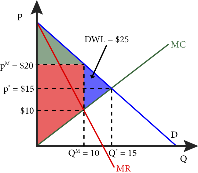
We can see from Figure 14.4.2 that the dead weight loss is a triangle with a base of 10, because at QM=10, MC=$10 and pM=$20, therefore the distance between the two is $10, and a height of 5, the difference between QM and Q*. Using the formula for the area of a triangle of ½ base times height, we get ½($10)(5) = $25.
SUMMARY
Review: Topics and Related Learning Outcomes
14.1 Conditions for Monopoly
Learning Objective 14.1: Explain the conditions that lead to monopolies.
14.2 Profit Maximization for Monopolists
Learning Objective 14.2: Explain how monopolists maximize profits and solve for the optimal monopolist’s solution from a demand curve and a marginal cost curve.
14.3 Market Power and the Demand Curve
Learning Objective 14.3: Describe the relationship between demand elasticity and a monopolist’s ability to price above marginal cost.
14.4 Monopoly and Welfare
Learning Objective 14.4: Describe the how monopolists create deadweight loss and explain how deadweight loss affects societal welfare.
Learn: Key Terms and Graphs
Terms
Graphs
Monopoly, Revenue and Marginal Revenue
Demand, Marginal Revenue and Total Revenue
Profit Maximization for a Monopolist
Solution to Tesla’s Profit Maximization Problem
Supplemental Resources
Practice Questions
YouTube Videos
These videos from the YouTube channel ‘Department of Economics’ may be helpful.
Policy Example
Policy Example: Should the Government Give Patent Protection to Companies That Make Live-Saving Drugs?
Learning Objective: Explain the effect of patent protection on drug markets and the trade-off society makes to promote the development of new drugs.
Providing companies like AstraZeneca patent protection for drugs like Crestor gives them a profit incentive to invest in the research and development of new, medically important, drugs. However, from 14.4 we also know that monopoly power creates deadweight loss. Figure 1 shows the deadweight loss that results from monopoly power, but it is important to understand what the deadweight loss represents: this is the loss to society that results from the reduction in output of these medically important drugs. By restricting output, monopolies keep prices high and in so doing exclude a segment of consumers who would purchase the drugs if the price were at marginal cost as would be the case in a perfectly competitive market.
Figure 1: Deadweight Loss From Monopoly Power
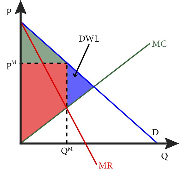
However, there would be an even larger deadweight loss if the drug was never discovered and the market never created. The total surplus, the combination of the red and green shaded areas in Figure 1, would be lost.
The most basic policy question is therefore whether the benefit to society is greater then the deadweight loss. Given diagram in Figure 1 the answer is almost certainly yes. Another policy question is whether there is an alternate policy that could achieve the same objective of developing new medicines at a lower societal cost – the most obvious is to fund the research of new medicines directly by government and then allow new discoveries to be produces by many firms. This would lead to more production and lower costs of new drugs but might not be as efficient at promoting new discoveries. A final question is whether the patent protections promote the discovery of only the most profitable drugs, such as those often associated with aging in high-income countries. Malaria, a disease that remains one of the most lethal in the world, has not generated a lot of funding into the creation of a new drug to combat it and many critics believe this is because it is a disease most commonly found in low-income countries and thus the potential profits are low because the market could not support high prices. Supporters of the current system like the fact that is it private enterprise, not government, that decides in which areas to invest resources thus ensuring that the drugs with the highest expected benefit are invested in most heavily.
Candela Citations
- Authored by: Joel Bruneau & Clinton Mahoney. License: CC BY-NC-SA: Attribution-NonCommercial-ShareAlike
- Module 15: Monopoly. Authored by: Patrick Emerson. Retrieved from: https://open.oregonstate.education/intermediatemicroeconomics/chapter/module-15/. License: CC BY-NC-SA: Attribution-NonCommercial-ShareAlike
- Elasticity. Authored by: Preston McAfee & Tracy R Lewis. Retrieved from: https://resources.saylor.org/wwwresources/archived/site/textbooks/Introduction%20to%20Economic%20Analysis.pdf. License: CC BY-NC-SA: Attribution-NonCommercial-ShareAlike
- Sources of Monopoly. Authored by: Preston McAfee & Tracy R Lewis. Retrieved from: https://resources.saylor.org/wwwresources/archived/site/textbooks/Introduction%20to%20Economic%20Analysis.pdf. License: CC BY-NC-SA: Attribution-NonCommercial-ShareAlike
- Basic Analysis. Authored by: Preston McAfee & Tracy R Lewis. Retrieved from: https://resources.saylor.org/wwwresources/archived/site/textbooks/Introduction%20to%20Economic%20Analysis.pdf. License: CC BY-NC-SA: Attribution-NonCommercial-ShareAlike
- Module 16: Pricing Strategies. Authored by: Patrick Emerson. Retrieved from: https://open.oregonstate.education/intermediatemicroeconomics/chapter/module-16/. License: CC BY-NC-SA: Attribution-NonCommercial-ShareAlike
is the sole supplier of a good for which there does not exist a close substitute
when one firm can supply the market more cheaply than two or more firms
an exclusive right to an invention, which excludes others from making, using, selling or importing it into the country for a limited time
is the the demand curve expressed with price as a function of quantity
the ability to choose a price above marginal cost; monopolists face downward sloping demand curves because they are the only supplier of a particular good or service and the market demand curve is therefore the monopolist’s demand curve
the percentage amount the price is above marginal cost
this index is used to measure the firm’s optimal markup; this is also a measure of market power as firms with more market power are more able to change prices above marginal cost
