
3
Joel Bruneau and Clinton Mahoney
Learning Objectives
- Define a budget constraint, conceptually, mathematically, and graphically
- Interpret the slope of the budget line
- Illustrate how changes in prices and income alter the budget constraint and budget line
- Illustrate how coupons, vouchers, and taxes alter the budget constraint and budget line
Module 3 – Budget Constraint
The Policy Question: Hybrid Car Purchase Tax Credit—Is it the Government’s Best Choice to Reduce Fuel Consumption and Carbon Emissions?
The U.S. government policy of extending tax credits toward the purchase of electric and hybrid cars can have consequence beyond decreasing carbon emissions. For instance, a consumer that purchases a hybrid car could spend less money on gas and have more money to spend on other things. This has implications for both the individual consumer and the larger economy.
Even the richest people – from Bill Gates to Oprah Winfrey – can’t afford to own everything in the world. Each of us has a budget that limits the extent of our consumption. Economists call this limit a budget constraint. In our policy example, an individual’s choice between consuming gasoline and everything else is constrained by his or her current income. Any additional money spent on gasoline is money that is not available for other goods and services and vice-versa. This is why the budget constraint is called a constraint.
The budget constraint is governed by income on the one hand, how much money a consumer has available to spend on consumption, and the prices of the goods the consumer purchases on the other.
Exploring the Policy Question
What are some of the budget implications for a consumer who owns a hybrid car? What purchase decisions might this consumer make given his or her savings on gas, and how does this, in turn, affect the goals of the tax subsidy policy?
3.1 Description of the Budget Constraint
LO1: Define a budget constraint, conceptually, mathematically, and graphically.
3.2 The Slope of the Budget Line
LO2: Interpret the slope of the budget line.
3.3 Changes in Prices and Income
LO3: Illustrate how changes in prices and income alter the budget constraint and budget line.
3.4 Coupons, Vouchers, and Taxes
LO4: Illustrate how coupons, vouchers, and taxes alter the budget constraint and budget line.
3.1 Description of the Budget Constraint
LO1: Define a budget constraint, conceptually, mathematically, and graphically.
The budget constraint is the set of all the bundles a consumer can afford given that consumer’s income. We assume that the consumer has a budget – an amount of money available to spend on bundles. For now, we do not worry about where this money or income comes from, we just assume a consumer has a budget.
So what can a consumer afford? Answering this depends on the prices of the goods in question. Suppose you go to the campus store to purchase energy bars and vitamin water. If you have $5 to spend, energy bars cost fifty cents each, and vitamin water costs $1 a bottle, then you could buy 10 bars, and no vitamin water, no bars and 5 bottles of vitamin water, 4 bars and 2 vitamin waters and so on.
This table shows the possible combinations of energy bars and vitamin water the student can buy for exactly $5:
|
Energy Bars |
Bottles of Vitamin Water |
|
10 |
0 |
|
8 |
1 |
|
6 |
2 |
|
4 |
3 |
|
2 |
4 |
|
0 |
5 |
It is also true that you could spend less than $5 and have money left over. So we have to consider all possible bundles −including consuming none at all.
Note that we are focusing on bundles of two goods so that we maintain tractability (as explained in module 1), but it is simple to think beyond two goods by defining one of the goods as “money spent on everything else.”
Mathematically, the total amount the consumer spends on two goods, A and B, is:
(3.1) , [latex]P_{A}A+P_{B}B[/latex]
where [latex]P_{A}[/latex] is the price of good A and [latex]P_{B}[/latex] is the price of good B. If the money the consumer has to spend on the two goods, his income, is given as I, then the budget constraint is:
(3.2)[latex]P_{A}A+P_{B}B\geq I[/latex]
Note the inequality: This equation states that the consumer cannot spend more than his income but can spend less. We can simplify this assumption by restricting the consumer to spending all of his income on the two goods. This will allow us to focus on the frontier of the budget constraint. As we shall see in Module 4, this assumption is consistent with the more-is-better assumption – if you can consume more (if your income allows it) you should because you will make yourself better off. With this assumption in place, we can write the budget constraint as:
(3.3)[latex]P_{A}A+P_{B}B=I[/latex]
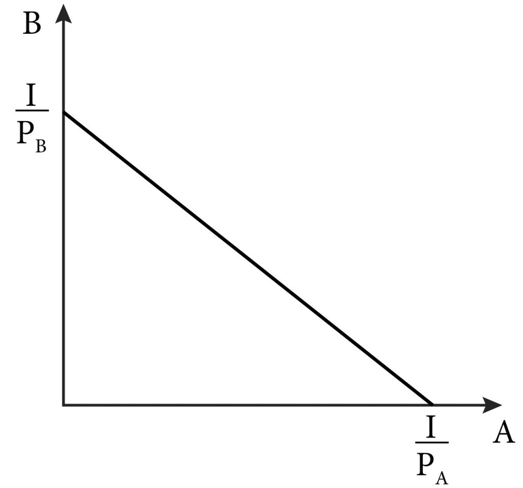
Graphically, we can represent this budget constraint as in Figure 3.1. We call this the budget line: The line that indicates the possible bundles the consumer can buy when spending all his income.
Figure 3.1 The budget line is the graph of the budget constraint equation (3.3).
LO2: Interpret the slope of the budget line
From the graph of the budget constraint in section 3.1, we can see that the budget line slopes downward and has a constant slope along its entire length. This makes intuitive sense: If you buy more of one good, you are going to have to buy less of the other good. The rate at which you can trade one for the other is determined by the prices of the two goods, and they don’t change.
We can see these details in Figure 3.2
Figure 3.2 Intercepts and slope for the budget line

We can find the slope of the budget line easily by rearranging equation (3.3) so that we isolate B on one side. Note that in our graph, B is the good on the vertical axis, so we will rearrange our equation to look like a standard function with B as the dependent variable:
(3.4) [latex]B=\frac{I}{P_{B}}-\frac{P_{A}}{P_{B}}A[/latex]
Now, we have our budget line represented in point-slope form where:
The first part, [latex]\frac{I}{P_{B}}[/latex], is the vertical intercept.
The second part,[latex]-\frac{P_{A}}{P_{B}}[/latex] , is the slope coefficient on A.
Note that the slope of the budget line is simply the ratio of the prices, also known as the price ratio. This is the rate at which you can trade one good for the other in the marketplace. To see this, let’s return to the campus store with $5 to spend on energy bars and vitamin water.
Suppose you originally decided to buy 5 bottles of vitamin water and placed them in a basket. After some thought, you decided to trade 1 bottle for 2 energy bars. Now you have 4 bottles of vitamin water and 2 energy bars in the basket. If you want even more bars, the same trade off is available: 2 more bars can be had if you give up one bottle of vitamin water, and so on.
The slope of the budget line is also called the economic rate of substitution (ERS).
The slope of the budget line also represents the opportunity cost of consuming more of good A because it describes how much of good B the consumer has to give up to consume one more unit of good A. The opportunity cost of something is the value of the next-best alternative given up in order to do get it. For example, if you decide to buy one more bottle of vitamin water, you have to give up two energy bars. Note that opportunity cost is not limited to the consumption of material goods. For example, the opportunity cost of an hour’s nap might be the hour of studying microeconomics that did not happen because of it.
Changes in Prices and Income
LO3: Illustrate how changes in prices and income alter the budget constraint and budget line.
From our mathematical description of the budget line, we can easily see how changes in prices and income affect the budget line and a consumer’s choice set —the set of all the bundles available to her at current prices and income. Let’s go back to equation (3.3):
(3.5)[latex]P_{A}A+P_{B}B=I[/latex]
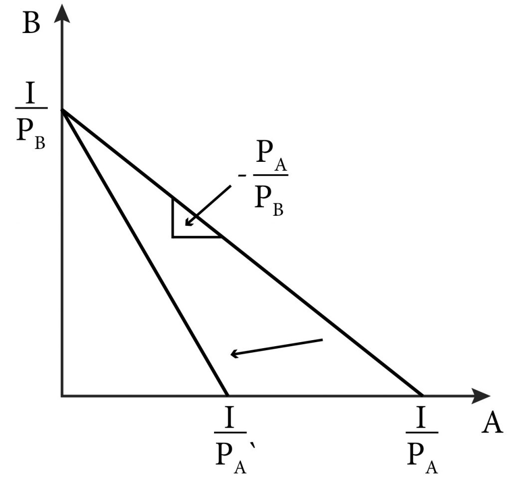
We know from the previous Figure 3.3 that the vertical intercept for equation (3.3) is [latex]\frac{I}{P_{B}}[/latex] and the horizontal intercept is [latex]\frac{I}{P_{A}}[/latex].
Now consider an increase in the price of good A. Notice in Figure 3.3 that this increase does not affect the vertical intercept, only the horizontal intercept. As [latex]P_{A}[/latex] increases,[latex]\frac{I}{P_{A}}[/latex] decreases, moving closer to the origin. This change makes the budget line ‘steeper’ or more negatively sloped as we can see from the slope coefficient: [latex]-\frac{P_{A}}{P_{B}}[/latex]. As [latex]P_{A}[/latex] increases, this ratio increases in absolute value, so the slope becomes more negative or steeper. What this means intuitively is that the trade-off or opportunity cost has risen. Now, the consumer has to give up more of good B to consume one more unit of good A.
Figure 3.3 Changing the price of one good changes the slope of the budget line.
Next, consider a change in income. Suppose the consumer gets an additional amount of money to spend, so I increases. I affects both intercept terms positively, so as I increases both [latex]\frac{I}{P_{B}}[/latex] and [latex]\frac{I}{P_{A}}[/latex] increase or move away from the origin. But I does not affect the slope: [latex]-\frac{P_{A}}{P_{B}}[/latex]. Thus the shift in the budget line is a parallel shift outward – the consumer with the additional income can afford more of both.
4 Coupons, Taxes, and Vouchers
LO4: Illustrate how coupons, vouchers and taxes alter the budget constraint and budget line.
Budget constraints can change due to changes in prices and income, but let’s now consider other common features of the real-world market that can affect the budget constraint. We start with coupons or other methods firms use to give discounts to consumers.
Consider a coupon or a sale that gives consumers a discount on the price of one item in our budget constraint problem. A coupon that entitles the bearer to a percentage off in price is essentially a reduction in price and has precisely the same effect. For example, a 20% off coupon on a good that normally costs $10 is the same as reducing the price to $8.
More complicated is a coupon that gives a percentage off the entire purchase. In this case, the percentage is taken from the price of both items A and B in our budget constraint problem. In this case, the price ratio, or the slope of the budget constraint, does not change.
For example, if the price of A is regularly $10 and the price of B is regularly $20 then with 20% off the entire purchase, the new prices are $8 and $16 respectively. Intuitively, we can see that this is equivalent to increasing the income, and achieves the same result: by expanding the budget set, the consumer can now afford bundles with more of both goods.
|
Product |
Regular Price |
New Price with 20% discount on entire purchase |
|
A |
$10 |
$8 |
|
B |
$20 |
$16 |
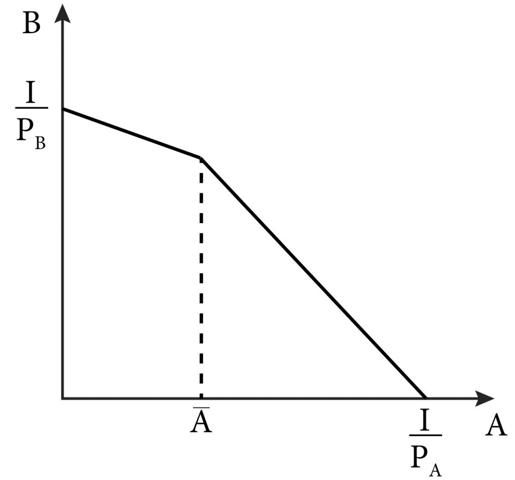
Another common discount is on a maximum number of items. For example, you might see an advertisement for 20% off up to three units of good A. This discount lowers the opportunity cost of A in terms of B for the first three units, but reverts back to the original opportunity cost thereafter. Figure 3.4 illustrates this.
Figure 3.4 The effect of a discount on the first A̅ units of A.
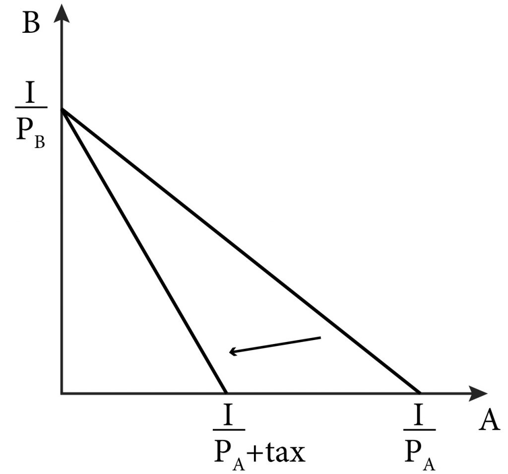
Taxes have the same effects as coupons but in the opposite direction. An ad valorem tax is a tax based on the value of a good, such as a percentage sales tax. In terms of the budget constraint, an ad valorem tax on a specific good is equivalent to an increase in price, as shown in Figure 3.5. A general sales tax on all goods has the effect of a parallel shift of the budget line inward. Note also that income taxes are, in this case, functionally equivalent to a general sales tax, they cause a parallel shift inward of the budget line.
Figure 3.5 An ad valorem tax changes the slope and horizontal intercept of the budget line.
Vouchers that entitle the bearer to a certain quantity of a good (either value or quantity) are slightly more complicated. Let’s return to your purchase of vitamin water and energy bars. Suppose you have a voucher for 2 free energy bars.
You have $5
The price of 1 energy bar is $0.50
The price of 1 bottle of vitamin water is $1.
How would we now draw your budget line?
One place to start is to consider the simple bundle that contains2 energy bars and 2 bottles of vitamin water. Note that giving up 1 or 2 bars does not allow the student to consume any more vitamin water. The opportunity cost of these 2 bars is 0, and so the budget line in this part has a 0 slope. After using the voucher, if the student wants more than 2 bars the opportunity cost is the same as before – .05 a bottle of vitamin water – and so the budget line from this point on is the same as before. The new budget line with the voucher has a kink.
SUMMARY
Review: Topics and Related Learning Outcomes
3.1 Description of the Budget Constraint
LO1: Define a budget constraint
3.2 The Slope of the Budget Line
LO2: Discuss the interpretation of the slope of the budget line
3.3 Changes in Prices and Income
LO3: Illustrate how changes in prices and income alter the budget constraint and budget line
3.4 Coupons, Vouchers and Taxes
LO4: Illustrate how coupons, vouchers and taxes alter the budget constraint and budget line
Learn: Key Terms and Graphs
Terms
Economic Rate of Substitution (ERS)
Graphs
Equations
Supplemental Resources
Practice Questions
YouTube Videos
This video from the YouTube channel ‘Department of Economics’ may be helpful.
Policy Example
Policy Example: The Hybrid Car Subsidy and Consumers’ Budgets
For several modules, we have considered the policy of a hybrid car tax credit. In Module 1, we thought about various driving preferences of a typical consumer. In Module 2, we translated these preferences into a type of utility function and corresponding indifference curve. Now, let’s think about the appropriate budget line for our policy example.
To start, let’s use the same two axes as we used for the indifference curve map as shown in Figure 1. In other words, let’s place ‘miles driven’ on the horizontal axis and $, which is all the money spent on other consumption on the vertical axis. For now, we won’t specify the precise level of income..
Now we can ask, what is the price of ‘other consumption?’ Since we are talking about money left over after paying for miles driven, the price for other consumption is simply 1. This is because we are talking about money itself and the price of a dollar is a dollar. So, the intercept on this axis is simply the value of I.
But what is the price of a mile driven? This question is more complicated and includes the cost of maintenance and depreciation. However, because we are focused on the effect of increasing the miles per gallon of gas, let’s concentrate on only the cost as it relates to the purchase of gasoline. In this case, the cost of driving a mile is the price of gasoline divided by the car’s miles per gallon (MPG). Since we are again interested not in an individual but a group, we can use the average price of a gallon of regular gas divided by the average MPG of cars driven in the United States as a reasonable approximation of the cost of a mile driven in a non-hybrid cr. Now we have the ‘price’ of driving a mile; dividing income by this price gives us the intercept on the ‘miles driven’ axis.
Figure 1 A consumer’s budget constraint for the hybrid car policy
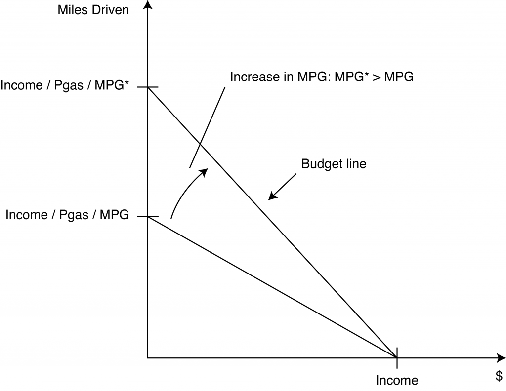
Now that we have a budget constraint for our electric and hybrid car subsidy policy example, we can see the effect of the policy on the constraint. Doubling the MPG from 20, say, to 40, dramatically reduces the price of driving a mile . This reduction causes the ‘miles driven’ intercept to move upwards and the entire budget constraint to move outward. Note that now the typical consumer can afford to consume bundles with more of both miles driven and everything else – bundles that were unavailable to them prior to the policy.
Equation (1) summarizes the budget constraint for miles driven and other goods.
(1) Income = (PMiles Driven)(Miles Driven) + Dollars Spent on Other Consumption
Exploring the Policy Questions
- What can we say about the availability of bundles after the hybrid car tax credit is enacted compared to before? Do the bundles represent more consumption of only miles driven or do they represent more of other goods as well?
- Another type of car that is high mileage (high MPG) is a diesel car. In the United States, however, the price of diesel gas is typically higher than the price of regular gas. How would only higher MPG shift the budget line in Figure 1? How would only higher priced gas shift the budget line in figure 1? How would these two factors together alter the budget line from Figure 1?
- If the government subsidizes the purchase of hybrid cars through a rebate that adds to the income of consumers, what happens to the budget line in Figure 1?
Candela Citations
- Authored by: Joel Bruneau & Clinton Mahoney. License: CC BY-NC-SA: Attribution-NonCommercial-ShareAlike
- Module 3: Budget Constraint. Authored by: Patrick Emerson. Retrieved from: https://open.oregonstate.education/intermediatemicroeconomics/chapter/module-3/. License: CC BY-NC-SA: Attribution-NonCommercial-ShareAlike
- 12.2 Budget or Feasible Set. Authored by: Preston McAfee & Tracy R Lewis. Retrieved from: https://resources.saylor.org/wwwresources/archived/site/textbooks/Introduction%20to%20Economic%20Analysis.pdf. License: CC BY-NC-SA: Attribution-NonCommercial-ShareAlike
is the set of all the bundles a consumer can afford given that consumer’s income
is the line on a graph that indicates all of the possible bundles the consumer can buy when spending all their income
is the rate at which you can trade one good for the other in the marketplace; this is the slope of the budget line on a graph
is another term for the slope of the budget line
the opportunity cost of something is the value of the next-best alternative given up in order to do get it
is a tax based on the value of a good, such as a percentage sales tax
