
1
Joel Bruneau and Clinton Mahoney
Learning Objectives
- List and explain the three fundamental assumptions about preferences
- Define and draw an indifference curve
- Relate the properties of indifference curves to assumptions about preference
- Define marginal rate of substitution
- Use indifference curves to illustrate perfect complements and perfect substitutes
Module 1: Preferences and Indifference Curves

The Policy Question: Is a Tax Credit on Hybrid Car Purchases the Government’s Best Choice to Reduce Fuel Consumption and Carbon Emissions?
The U.S. government, concerned about the dependence on imported foreign oil and the release of carbon into the atmosphere, has enacted policies where consumers can receive substantial tax credits toward the purchase of certain models of all-electric and hybrid cars.
This credit may seem like a good policy choice but it is a costly one, it takes away resources that could be spent on other government policies, and it is not the only approach to decreasing carbon emissions and dependency on fossil fuels. So how do we decide which policy is best?
Suppose that this tax credit is wildly successful and doubles the average fuel economy of all cars on U.S. roads (this is clearly not realistic but useful for our subsequent discussions). What do you think would happen to the fuel consumption of all U.S. motorists? Should the government expect fuel consumption and carbon emissions of U.S. cars to decrease by half in response?
The answers to these questions are critical when choosing among the policy alternatives. In other words, is offering a subsidy to consumers the most effective way to meet the policy goals of decreased dependency on foreign oil and carbon emissions? Are there more efficient—that is, less expensive–ways to achieve these goals? The ability to predict with some accuracy the response of consumers to this policy is vital to determining the merits of the policy before millions of federal dollars are spent.
Consumption decisions, such as how much automobile fuel to consume, come fundamentally from preferences – our likes and dislikes. Human decision making, driven by our preferences, is at the core of economic theory. Since we can’t consume everything our hearts desire, we have to make choices and those choices are based on our preferences. Choosing based on likes and dislikes does not mean that we are selfish–our preferences may include charitable giving and the happiness of others.
In this module, we will study preferences in economics.
1.1 Fundamental Assumptions about Individual Preferences
Learning Objective 1.1: List and explain the three fundamental assumptions about preferences.
1.2 Graphing Preferences with Indifference Curves
Learning Objective 1.2: Define and draw an indifference curve.
1.3 Properties of Indifference Curves
Learning Objective 1.3: Relate the properties of indifference curves to assumptions about preference
1.4 Marginal Rate of Substitution
Learning Objective 1.4: Define marginal rate of substitution.
1.5 Perfect Complements and Perfect Substitutes
Learning Objective 1.5: Use indifference curves to illustrate perfect complements and perfect substitutes.
1.1 Fundamental Assumptions about Individual Preferences
Learning Objective 1.1: List and explain the three fundamental assumptions about preferences.
To build a model that can predict choices when variables change, we need to make some assumptions about the preferences that drive consumer choices.
Economics makes three assumptions about preferences that are the most basic building blocks of our theory of consumer choice.
To introduce these it is useful to think of collections or bundles of goods. To simplify, let’s identify two bundles, A and B. The way we think of preferences always boils down to comparing two bundles. Even if we are choosing among three or more bundles, we can always proceed by comparing pairs and eliminating the lesser bundle until we are left with our choice.
When we call something a good, we mean exactly that – something that a consumer likes and enjoys consuming. Something that a consumer might not like we call a bad. The fewer bads consumed, the happier a consumer is. To keep things simple, we will focus only on goods, but it is easy to incorporate bads into the same framework by considering their absence – the fewer the bads the better.
The three fundamental assumptions about preferences are:
- Completeness: We say preferences are complete when a consumer can always say one of the following about two bundles: A is preferred to B, B is preferred to A or A is equally good as B
- Transitivity: We say preferences are transitive if they are internally consistent: if A is preferred to B and B is preferred to C, then it must be that A is preferred to C.
- More is Better: If bundle A represents more of at least one good, and no less of any other good, then bundle A is preferred to B. This is often referred to as strict monotonicity of preferences.
The most important results of our model of consumer behavior hold when we only assume completeness and transitivity, but life is much easier if we assume more is better as well. If we assume free disposal (we can get rid of extra goods at no cost) the assumption that more is better seems reasonable. It is certainly the case the more is not worse in that situation and so to keep things simple we’ll maintain the standard assumption that we prefer more of a good to less.
Our model works well when these assumptions are valid, which seems to be most of the time in most situations. However, sometimes these assumptions do not apply. For instance, in order to have complete and transitive preferences, we must know something about the goods in the bundle. Imagine an American who does not speak Hindi entering an Indian restaurant where the menu is entirely in Hindi. Without the aid of translation, the customer cannot act as economic theory would predict.
1.2 Graphing Preferences with Indifference Curves
Learning Objective 1.2: Define and draw an indifference curve.
Individual preferences, given the basic assumptions, can be represented using something called indifference curves. An indifference curve is a graph of all of the combinations of bundles that a consumer prefers equally. In other words the consumer would be just as happy consuming any of them. Representing preferences graphically is a great way to understand both preferences and how the consumer choice model works – so it is worth mastering them early in your study of microeconomics.
Bundles can contain many goods, but to simplify, we will consider only pairs of goods. At first this may seem impossibly restrictive but it turns out that we don’t really lose generality in so doing. We can always consider one good in the pair to be, collectively, all other consumption goods. What the two-good restriction does so well is to help us see the tradeoffs in consuming more of one good and less of another.
Figure 1.2.1 Bundles and Indifference Curves
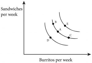
Figure 1.2.1 is a graph with two goods on the axes: the weekly consumption of burritos and the weekly consumption of sandwiches for a college student. In the middle of the graph is point A, which represents a bundle of both burritos (read from the horizontal axis) and sandwiches (read from the vertical axis).
Now we can ask what bundles are better, worse or the same in terms of satisfying to this college student. Clearly bundles that contain less of both goods, like bundle D, are worse than A, B or C because they violate the more is better assumption. Equally clear is that bundles that contain more of both goods, like bundle E are better than A, B, C and D because they satisfy the more is better assumption.
To create an indifference curve we want to identify bundles that this college student is indifferent about consuming. If a bundle has more burritos the student would have to have fewer sandwiches and vice versa. By finding all the bundles that are just as good as A, like B and C, and connecting them with a line, we create an indifference curve like the one in the middle.
Notice that Figure 1.2.1 includes several indifference curves. Each curve represents a different level of overall satisfaction that the student can achieve via burrito/sandwich bundles. A curve further out from the origin represents a higher level of satisfaction than a curve closer to the origin.
Notice also that these curves share a number of characteristics: they slope downward, they do not cross and they are all bowed in. We explore these properties in more detail in the next section.
1.3 Properties of Indifference Curves
Learning Objective 1.3: Relate the properties of indifference curves to assumptions about preference.
As introduced in Section 1.2, well-behaved indifference curves have three key properties:
- they are downward sloping
- they do not cross
- they are bowed in (a non-technical way of saying they are strictly convex to the origin).
For simplicity and clarity, from here on we will describe preferences that lead to indifference curves with these three properties as standard preferences. This will be our default assumption – that consumers have standard preferences unless otherwise noted. As we will see in this module, there are other types of preferences that are common as well and we will continue to study both the standard type and the other types as we progress through the material.
To understand the first two properties, it’s useful to think about what happen if they were not true.
Figure 1.3.1 Upward Sloping Indifference Curves Violate the More-is-Better Assumption
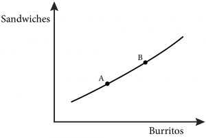
Think about indifference curves that slope upward as in figure 1.3.1. In this case we have two bundles on the same indifference curve, A and B but B has more of both burritos and sandwiches than does A. So this violates the assumption of more is better. More is better (or strict monotonicity of preferences) implies indifference curves are downward sloping.
Figure 1.3.2: Crossing Indifference Curves Violate the Transitivity Assumption
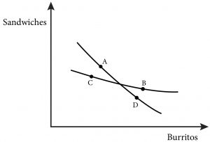
Similarly, consider Figure 1.3.2. In this figure there are two indifference curves that cross. Now consider bundle A on one of the indifference curves. It represents more of both goods than bundle C that lies on the other indifference curve. Because the bundle B lies on the same indifference curve as bundle C the two bundles should be equally preferred and therefore A should be preferred to B and C. B also represents more of both goods than bundle D and therefore B should be preferred to D. However D is on the same indifference curve as A, so B should be preferred to A. Since A can’t be preferred to B and B preferred to A at the same time, this is a violation of our assumptions of transitivity and more is better. Transitivity and more is better imply that indifference curves do not cross.
Now we come to the third property: indifference curves bow in. This property comes from a fourth assumption about preferences, which we can add to the assumptions discussed in Section 1.1:
- Preference for variety (or strictly convex preferences).
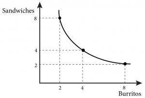
The assumption that consumers prefer variety is not necessary, but still applies in many situations. For example, most consumers would probably prefer to eat both sandwiches and burritos during a week and not just one or the other (remember this is for consumers who consider them both goods – who like them). In fact, if you had only sandwiches to eat for a week, you’d probably be willing to give up a lot of sandwiches for a few burritos and vice versa. Whereas if you had reasonably equal amounts of both you’d be willing to trade one for the other but at closer to 1 to 1 ratios. Notice that if we graph this we naturally get bowed in indifference curves, as shown in Figure 1.3.3. Preference for variety (or strictly convex preferences) implies indifference curves are bowed in.
Figure 1.3.3 Preference for Variety Means that Indifference Curves are Bowed In.
Remember these three key points about preferences and well-behaved indifference curves:
- More is better (or strictly monotonic preferences) implies indifference curves are downward sloping.
- Transitivity and more is better imply indifference curves do not cross.
- Preference for variety (or strictly convex preferences) implies indifference curves are bowed in.
Important Note: There is a distinction between both strictly vs. weakly monotonic preferences and strictly vs. weakly convex preferences which deserve mention. Whereas strictly monotonic preferences implies indifference curves must strictly slope downwards, weakly monotonic preferences may slope downwards, may have no slope, or may have a slope of (negative/positive) infinity – this is easiest to understand by saying ‘more is not worse’ instead of ‘more is better’ and arises from an assumption of free disposal of unwanted units of a good. Whereas strictly convex preferences implies indifferences curves are bowed in on a (usually smooth) rounded arc, weakly convex preferences may be bowed in on a (usually smoothly) rounded arc, or be a straight line with a downward slope – this is easiest to understand by saying the consumer is ‘indifferent about variety’ instead of saying the consumer has a ‘preference for variety’. We will see examples of these types of preferences in Figure 1.5.1 (Perfect Complements) and 1.5.2 (Perfect Substitutes).
1.4 Marginal Rate of Substitution
Learning Objective 1.4: Define marginal rate of substitution.
From now on we will assume that consumers like variety and that indifference curves are bowed in. However, it is worth considering examples on either extreme: perfect substitutes and perfect complements.
When we move along an indifference curve we can think of a consumer substituting one good for another. Two bundles on the same indifference curve, which represent the same satisfaction from consumption, have one thing in common: they represent more of one good and less of the other. This makes sense given our assumption of ‘more is better’; if more of one good makes you better off, then you must have less of the other good in order to maintain the same level of satisfaction.
In economics we have a more technical way of expressing this tradeoff: the marginal rate of substitution. The marginal rate of substitution (MRS) is the amount of one good a consumer is willing to give up to get one more unit of another good and maintain the same level of satisfaction. This is one of the most important concepts in economics because it is critical to understanding consumer choice.
Mathematically, we express the marginal rate of substitution for two generic goods like this:
[latex]MRS=\frac{\Delta A}{\Delta B}[/latex]
where Δ indicates a change in the quantity of the good.
In the case of our student consuming burritos and sandwiches, the expression would be:
[latex]MRS=\frac{\Delta Sandwiches }{\Delta Burritos}[/latex]
For example suppose at his current consumption bundle, 5 burritos and 4 sandwiches weekly, Luca is willing to give up 2 burritos to get one more sandwich. Another way of saying the same thing is that Luca is indifferent between consuming 5 burritos and 4 sandwiches in a week or 3 burritos and 5 sandwiches in a week. The MRS for Luca at that point is:
[latex]MRS=\frac{\Delta Sandwiches }{\Delta Burritos}=\frac{-2}{1}=-2[/latex]
Note that the MRS is negative because it represents a tradeoff: more sandwiches for fewer burritos.
Figure 1.4.1 illustrates the marginal rate of substitution for burritos and sandwiches graphically.
Figure 1.4.1 Marginal rate of substitution for burritos and sandwiches.
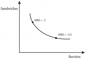
Notice that Figure 1.4.1 illustrates a change in the good on the vertical axis (sandwiches) over the change in the good on the horizontal axis (burritos). This is the same as saying the rise over the run. From this discussion and graph, it should be clear that the MRS is same as the slope of the indifference curve at any given point along it.
1.5 Perfect Complements and Perfect Substitutes
Learning Objective 1.5: Use indifference curves to illustrate perfect complements and perfect substitutes.
We have now studied the assumptions upon which our model of consumer behavior is built:
- completeness
- transitivity
- more is better
- love of variety
We have also seen how these assumptions govern the properties of indifference curves.
It is worth taking a moment to think about two other types of preference relations that are special cases but not uncommon: perfect complements and perfect substitutes.
Perfect Complements
Perfect complements are goods that consumers want to consume only in fixed proportions.
Consider the example of an iPod Shuffle and earphones. An iPod Shuffle is useless without earphones and earphones are useless without an iPod Shuffle, but put them together and, voila, you have a portable stereo, which is worth quite a lot. An extra set of earphones doesn’t increase the usefulness of the iPod and an extra iPod doesn’t increase the usefulness of the earphones. So these are things that we consume in a fixed proportion: one iPod goes with one set of earphones. We call such preference relations perfect complements.
Figure 1.5.1 illustrates the process of drawing indifference curves for perfect complements.
Figure 1.5.1: Indifference Curves for Goods that are Perfect Complements
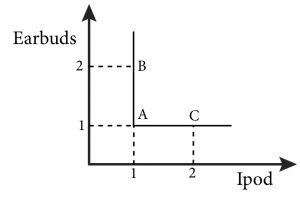
In Figure 1.5.1, when we start with a bundle of one iPod and one set of earbuds (as in bundle A), what are the other bundles that are just as good to the consumer? Two sets of earbuds and one iPod is no better than one set of earbuds and one iPod, so the bundle B lies on the same indifference curve. The same is true for two iPods and one set of earbuds, as in bundle C. From this example we can see that indifference curves for perfect complements have right angles.
Perfect Substitutes
Perfect substitutes are goods about which consumers are indifferent as to which to consume.
That is, one unit of one good is just as good as one unit of another good. Both Morton and Diamond Crystal are brands of table salt. For most consumers a teaspoon of one salt is just as good as a teaspoon of the other regardless of the amount possessed by the consumer. We call goods like these perfect substitutes.
Drawing indifference curves for perfect substitutes is straightforward as shown in Figure 1.5.2.
Figure 1.5.2: Indifference Curves for Goods that are Perfect Substitutes
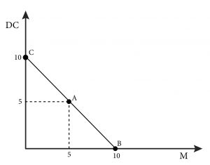
Bundle A in Figure 1.5.2 contains 5 teaspoons of each type of salt. This is just as good to the consumer as a bundle with 10 teaspoons of Morton salt and zero teaspoons of Diamond Crystal as in bundle B. It is also just as good as the 10 teaspoons of Diamond Crystal and zero teaspoons of Morton in bundle C.
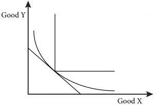
You can think of perfect complements and perfect substitutes as polar extremes of preference relations. Figure 1.5.3 shows how a typical indifference curve lies in between perfect complements and perfect substitutes. You should understand, when graphically represented, that the indifference curve for well behaved lies between perfect complements and perfect substitutes.
Figure 1.5.3: The Relationship between Indifference Curves for Well Behaved Preferences and Perfect Complements and Substitutes
SUMMARY
Review: Topics and Related Learning Outcomes
1.1 Fundamental Assumptions about Individual Preferences
Learning Objective 1.1: List and explain the three fundamental assumptions about preferences.
1.2 Graphing Preferences with Indifference Curves
Learning Objective 1.2: Define and draw an indifference curve.
1.3 Properties of Indifference Curves
Learning Objective 1.3: Relate the properties of indifference curves to assumptions about preference.
1.4 Marginal Rate of Substitution
Learning Objective 1.4: Define marginal rate of substitution.
1.5 Perfect Complements and Perfect Substitutes
Learning Objective 1.5: Use indifference curves to illustrate perfect complements and perfect substitutes.
Learn: Key Terms and Graphs
Terms
Well-behaved indifference curves
Marginal rate of substitution (MRS)
Graphs
Equations
[latex]MRS=\frac{\Delta A}{\Delta B}[/latex]
Supplemental Resources
YouTube Videos
These videos from the YouTube channel ‘Department of Economics’ may be helpful.
Policy Example
Policy Example: The Hybrid Car Tax Credit and Consumer Preference
The issue of consumer preferences is central to the real world policy question posed at the beginning of this module.

Recall that we are assuming that the tax credit will cause the average fuel economy of U.S. cars to double. So, from a consumer behavior perspective, one of the things we want to know in evaluating the policy is whether this improvement in gas mileage will cause an equivalent decrease in the demand for gasoline. In other words, the consumer decision is about the tradeoff of purchasing gasoline to travel in a car versus all of the other uses of the money spent on gas.
We can apply the principle of preferences and the assumptions we make about them to this particular question by drawing indifference curves, as shown in Figure 1.6.1
Figure 1: Indifference Curve for Miles Drives versus Money Spent on All Other Goods
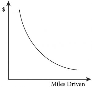
We can label one axis of the indifference curve map “miles driven” and the other “money for other consumption.” Doing so illustrates how confining ourselves to only two dimensions is really not that confining at all. By considering the other axis as money for all other purchases we are really looking at the general trade off between one particular consumption good and everything else that a consumer could possibly consume.
So, what would our indifference curve look like? As before it would be downward sloping – surely travelling more by car affords the consumer more freedom of movement and therefore more consumption choices, both of which are a good. The indifference curves would not cross for the same reasons discussed in section 1.3. But what about the principle of more is better? The point here is to again think about the principle of free disposal: as long as the ability to drive more miles is not bad (and it is hard to imagine how it could be) then more miles are never worse.
The remaining question is whether the preference for variety is a good assumption in this case. It is helpful to consider the extremes: for those consumers who own cars, never driving any miles is probably not very practical. Likewise spending one’s entire income only on expenses relating to driving one’s car is unappealing. A good assumption, then, is that most people with a car would prefer some combination of miles driven and other consumption to either extreme and we can draw our indifference curves as convex to the origin.
We are not yet in a position to say much about the policy itself, but we have one piece of the model we will use to analyze it. With this indifference curve we can move on to the other pieces of the model that we will study in Modules 2, 3 and 4.
Exploring the Policy Question
- Suppose that a typical consumer is concerned about how his or her individual driving habits are negatively impacting the environment. How might such a change in attitude change the shape of the consumer’s indifference curves?
Just for Fun
Candela Citations
- Module 1: Preferences and Indifference Curves. Authored by: Joel Bruneau & Clinton Mahoney. License: CC BY-NC-SA: Attribution-NonCommercial-ShareAlike
- Module 1: Preferences and Indifference Curves. Authored by: Patrick Emerson. Retrieved from: https://open.oregonstate.education/intermediatemicroeconomics/chapter/module-1/. License: CC BY-NC-SA: Attribution-NonCommercial-ShareAlike
We say preferences are complete when a consumer can always say one of the following about two bundles: A is preferred to B, B is preferred to A, or A is equally as good as B
We say preferences are transitive if they are internally consistent: if A is preferred to B and B is preferred to C, then it must be that A is preferred to C
If bundle A represents more of at least one good, and no less of any other good, then bundle A is preferred to B. This is often referred to as monotonicity of preferences.
a graph of all of the combinations of bundles that a consumer prefers equally
indifference curves that have the following graphical properties: (1) They are downward sloping; (2) They do not cross; (3) They are bowed in to the origin.
implies that indifference curves are bowed in; this is often referred to as convex preferences.
is the amount of one good a consumer is willing to give up to get one more unit of another good and maintain the same level of satisfaction
are goods that consumers want to consume only in fixed proportions
are goods about which consumers are indifferent as to which to consume
