
11
Joel Bruneau and Clinton Mahoney
Learning Objectives
- Identify the characteristics of a market
- Determine the equilibrium price and quantity for a market, both graphically and mathematically
- Calculate and graph excess supply and excess demand
- Calculate consumer surplus, producer surplus, and deadweight loss for a market
Module 11: Market Equilibrium – Supply and Demand
The Policy Question: Should government provide public marketplaces?

In the Capitol Hill neighbourhood of Washington, D.C., the Eastern Market is a large building and grounds, owned and operated by the city government. Farmers, bakers, cheese makers and other merchants of food, arts and crafts assemble there to sell their wares. Marketplaces like it were once a common feature of cities in the United States and Europe, but are now a relative rarity. Many have disappeared as citizens question government support of marketplaces.
So why does the government play a role in providing some markets? The answer is found in the way markets create benefits for the citizens they serve. In this module, we explore how prices and quantities are set in market equilibrium, how changes in supply and demand factors cause market equilibrium to adjust and how we measure the benefit of markets to society.
Markets are often private in the sense that the government is not involved in their creation or presence; instead they are generated by the desire of private individuals to engage in an exchange for a particular good. Sometimes, however, the government plays an active role in establishing and managing markets. At the end of the module we will study why this occurs, using the Eastern Market as an example.
Exploring the Policy Question
Is public investment in marketplaces justified and if so why?
11.1 What is a Market?
Learning Objective 11.1: Identify the characteristics of a market.
11.2 Market Equilibrium – The Supply and Demand Curves Together
Learning Objective 11.2: Determine the equilibrium price and quantity for a market, both graphically and mathematically.
11.3 Excess Supply and Demand
Learning Objective 11.3: Calculate and graph excess supply and excess demand.
11.4 Measuring Welfare and Pareto Efficiency
Learning Objective 11.4:
Calculate consumer surplus, producer surplus, and deadweight loss for a market.
11.1 What is a Market?
LO 11.1: Identify the characteristics of a market.
In Module 10 we found out where the market supply curve comes from – the cost structure of individual firms, which in turn comes from their technology as we discovered in Module 8. In Module 5 we found out where the demand curve comes from – the individual utility maximization problems of individual consumers. In both cases we assumed the demand for and supply of a specific good or service. In other words we were describing a particular market.
A market is characterized by a specific good or service being sold in a particular location at a defined time. So, for example, we might talk about:
- the market for eggs in Nashville, Tennessee in April of 2016.
- the market for rolled aluminum in the U.S. in 2015.
- the market for radiological diagnostic services worldwide in the last decade.
In addition, for whatever item, time and place we describe there must be both buyers and sellers in order for a market to exist. A market is where buyers and sellers exchange or where there is both demand and supply.
We tend to talk about markets somewhat loosely when studying economics. For example, we might discuss the market for orange juice and leave the time and place undefined in order to keep things simple. Or we might just say that we are looking at the market for denim jeans in the U.S. The difficulty with these simplifications is that we can lose sight of the basic assumptions about markets that are necessary for our analysis of them.
The six necessary assumptions for markets are the following:
- A market is for a single good or service.
- All goods or services bought and sold in a market are identical.
- The good or service sells for a single price.
- All consumers know everything about the product including how much they value it.
- There are many buyers and sellers and they are known to each other and can interact.
- All the costs and benefits of a transaction accrue only to the buyers and sellers who engage in it.
These assumptions are actually pretty easy to understand. They guarantee that the buyers who value the good more than it costs sellers to produce it will find a seller willing to sell to them. In other words there are no transactions that don’t happen because the buyer doesn’t know how much he or she likes the product or because a buyer can’t find a seller or vice-versa.
Of course, the assumptions describe an ideal market. In reality, many markets are not exactly like this, and later, in Section 7, we will examine what happens when these assumptions fail to hold.
11.2 Market Equilibrium: The Supply and Demand Curves Together
LO 11.2: Determine the equilibrium price and quantity for a market, both graphically and mathematically.
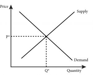
Economic equilibrium is a condition or state in which economic forces are balanced. In effect, economic variables remain unchanged from their equilibrium values in the absence of external influences (Investopedia 2022, https://www.investopedia.com/terms/e/economic-equilibrium.asp). Market equilibrium is the point where the quantity supplied by producers and the quantity demanded by consumers are equal. The only way the equilibrium changes is if an external event alters behaviour of consumers (a demand shock) or producers (a supply shock). When we put the demand and supply curves together we can determine the equilibrium price: the price at which the quantity demanded equals the quantity supplied. In Figure 11.2.1 the equilibrium price is shown as P* and it is precisely where the demand curve and supply curve cross. This makes sense–the demand curve gives the quantity demanded at every price and the supply curve gives the quantity supplied at every price so there is one price that they have in common, which is at the intersection of the two curves.
Figure 11.2.1: The Supply and Demand Curves and Market Equilibrium
Graphing the supply and demand curves to locate their intersection is one way to find the equilibrium price. We can also find this quantity mathematically. Consider a demand curve for stereo headphones that is described by the following function:
QD = 1800 – 20P
Note that in general we draw graphs of functions with the independent variable on the horizontal axis and the dependent variable on the vertical axis. In the case of supply and demand curves, however, we draw them with quantity on the horizontal axis and price on the vertical. Because of this, it is sometimes easier to express the demand relationship as an inverse demand curve: the demand curve expressed as price as a function of quantity. In our example this would be:
P = 90 – 0.05QD
This is just the original demand curve solved for P instead of QD. In the inverse demand curve the vertical intercept is easy to see from the equation: demand for headphones stops at the price of $90. No consumer is willing to pay $90 or more for headphones.
Similarly the supply curve can be represented as a mathematical function. For example, consider a supply curve described by the function:
QS = 50P – 1000
Similar to the demand curve we can express this as an inverse supply curve: the supply curve expressed as price as a function of quantity. In this case, the inverse supply curve would be:
P = 20 – 0.03QS
Here the vertical intercept, $20, gives us the minimum price to get a seller to sell headphones. At prices of $20 or less, there will be no supply. So we know that the equilibrium price should be between $20 and $90.
Solving for the equilibrium price and quantity is simply a matter of setting QD = QS and solving for the price that makes this equality happen. On our example setting QD = QS yields:
1800 – 20P = 50P – 1000
or
70P = 2800
or
P = $40
At P = $40, the quantity demanded and supplied can be found from the demand and supply curves:
QD = 1800 – 20(40) = 1000
QS = 50(40) – 1000 = 1000
That these two quantities match is no accident, this was the condition we set at the outset – that quantity supplied equals quantity demanded. So we know that a price of $40 per unit is the equilibrium price.
These supply and demand curves for headphones are graphed in Figure 11.2.2 below, and their intersection confirms the equilibrium price we calculated mathematically.
Figure 11.2.2: Explicit Supply and Demand Curves for Headphones
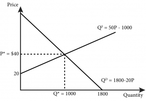
Note that we have also identified the equilibrium quantity, Q*—the quantity at which supply equals demand. At $40 per unit, 1000 headphones are demanded and exactly 1000 headphones are supplied. The equilibrium quantity has nothing to do with any kind of coordination or communication among the buyers and sellers; it has only to do with the price in the market. Seeing a unit price of $40, consumers demand 1000 units. Independently, sellers who see that price will choose to supply exactly 1000 units.
11.3 Excess Supply and Demand
LO 11.3: Calculate and graph excess supply and excess demand.
It makes sense that the equilibrium price is the one that equates quantity demanded with quantity supplied, but how does the market get to this equilibrium? Is this just an accident? No. The market price will automatically adjust to a point where supply matches demand. Excess supply or demand in a market will trigger such an adjustment.
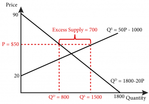
To understand this equilibrating feature of the market price, let’s return to our headphones example. Suppose the price is $50 instead of $40. At this price we know from the supply curve that 1500 units will be supplied to the market. Also, from the demand curve, we know that 800 units will be demanded. Thus there will be an excess supply of 700 units, as shown in Figure 11.2.3.
Excess supply occurs when, at a given price, firms supply more of a good than consumers demand. These are goods that have been produced by the firms that supply the market that have not found any willing buyers. Firms will want to sell these goods and know that by lowering the price more buyers will appear. So this excess supply of goods will lead to a lowering of the price. The price will continue to fall as long as the excess supply conditions exist. In other words, price will continue to fall until it reaches $40.
Figure 11.2.3: Excess Supply of Headphones at a Price of $50
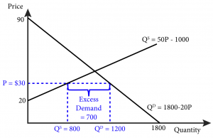
The same logic applies to situations where the price is below the intersection of supply and demand. Suppose the price of headphones is $30. We know from the demand curve that at this price, consumers will demand 1200 units. We also know from the supply curve that at this price suppliers will supply 500 units. So at $30 there will be excess demand of 700 units, as shown in Figure 11.2.3.
Excess demand occurs when, at a given price, consumers demand more of a good than firms supply. Consumers who are not able to find goods to purchase will offer more money in an effort to entice suppliers to supply more. Suppliers who are offered more money will increase supply and this will continue to happen as long as the price is below $40 and there is excess demand.
Figure 11.2.3 b: Excess Demand for Headphones at a Price of $30
Only at a price of $40 is the pressure for prices to rise or fall relieved and will the price remain constant.
11.4 Measuring Welfare and Pareto Efficiency
LO 11.4: Calculate consumer surplus, producer surplus, and deadweight loss for a market.
From our study of markets so far, it is clear that they can contribute to the economic well-being of both buyers and sellers. The term welfare, as it is used in economics, refers to the economic well-being of society as a whole, including producers and consumers. We can measure welfare for particular market situations.
To understand the economic concept of welfare—and how to quantify it–it is useful to think about the weekly farmers’ market in Ithaca, New York. The market is a place where local growers can sell their produce directly to consumers throughout the summer. It is very successful and many local residents go to the market to buy produce. Now consider the specific example of tomatoes. What is this market worth to the tomato sellers and buyers that transact in the market?
Suppose a farmer has a minimum willingness-to-accept price of $1 for an heirloom tomato. This price could be based on the farmer’s cost of production or the value she places on consuming the tomato herself. Suppose also that there is a consumer who really wants an heirloom tomato to add to his salad that evening and is willing to pay up to $3 for one. If these two people meet each other at the market and agree on a price of $2, how much benefit do they each get?
The seller receives $2 and it cost her $1 to provide the tomato, so she is $1 better off, the difference between what she received and what she would have accepted for the tomato. Likewise, the buyer pays $2 but receives $3 in benefit from the tomato, since that was his willingness to pay; his net benefit is the difference, or $1. The seller and buyer are both $1 better off because they had the opportunity to meet and transact. Without this opportunity the seller would have stayed at home with the tomato and been no better or worse off, and the buyer would not have a tomato for his salad but would be no better or worse off.
The difference between the price received and the willingness-to-accept price is called the producer surplus (PS). The difference between the willingness-to-pay price and the price paid is called the consumer surplus (CS). The sum of these two surpluses is called total surplus (TS). So the producer surplus in the tomato example is $1, the consumer surplus is $1 and the total surplus is $2. This is the surplus generated by the one transaction; if we add up all such transactions in the market we get a measure of the consumer and producer surplus from the market.
Quantifying surplus for an entire market is easy to do with a graph. Let’s return to our previous example of headphones and find the consumer and producer surplus.
Figure 11.4.1 shows that the consumer surplus is the area above the equilibrium price and below the demand curve –the green triangle in the figure. Similarly, the producer surplus is the area below the equilibrium price and above the supply curve –the red triangle in the figure. The area of each surplus triangle is easy to calculate using the formula for the area of a triangle: ½bh, where b is base and h is height.
Figure 11.4.1: Consumer Surplus and Producer Surplus in the Market for Headphones
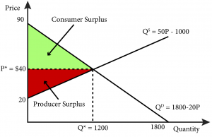
In the case of consumer surplus the triangle has a base of 1000, the distance from the origin to Q*, and a height of $50, the difference between $90, the vertical intercept and P*, which is $40.
Consumer surplus = ½(1000)($50) = $25,000
Similarly,
Producer surplus = ½(1000)($20)= $10,000
Total surplus created by this market is the sum of the two or $35,000. This is the measure of how much value the market creates through its enabling of these transactions. Without the ability to come together in this market the buyers and sellers would miss out on the opportunity to capture this surplus.
We say that a market is efficient when the entire potential surplus has been created. Such a market is an example of Pareto efficiency— an allocation of goods and services in which no redistribution can occur without making someone worse off. Think about the distribution of goods in the headphones example. All of the buyers and sellers that transact are made better off by the transaction because they gain some surplus from it. If they didn’t, they would not voluntarily trade. None of the trades that shouldn’t happen do. For example if there were more than 1000 units exchanged it would mean sellers were selling to buyers who valued the good less than the sellers’ cost of production, where the supply curve is above the demand curve, and one or both of the parties would be worse off because of the exchange.
Another way to see that the market equilibrium outcome is efficient is if we arbitrarily limit the number of goods exchanged to 900. Let’s call this maximum quantity restriction Q̅, where the bar above the Q indicates that it is fixed at that quantity. There are 100 surplus-creating transactions that don’t occur; this cannot be an efficient outcome because the entire potential surplus has not been created. The lost potential surplus has a name, deadweight loss (DWL): the loss of total surplus that occurs when there is an inefficient allocation of resources. The blue triangle in Figure 11.4.2 represents this deadweight loss.
Figure 11.4.2: Deadweight loss from a quantity constraint
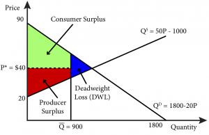
We can calculate the value of the deadweight loss precisely, again using the formula for the area of a triangle. Since the demand function is QD = 1800 – 20P, the point on the demand curve that results in a demand of 900 is a price of $45. Similarly the supply function is given as QS = 50P – 1000, the point on the supply curve that results in a quantity supplied of 900 is a price of $38. Thus the base of the triangle is $45-$38 or $7 and the height is the difference between the 1000 units that sold in the absence of a restriction and the 900 unit restricted quantity or 100. So DWL = ½($7)(100) = $350.
SUMMARY
Review: Topics and Related Learning Outcomes
11.1 What is a Market?
Learning Objective 11.1: Identify the characteristics of a market.
11.2 Market Equilibrium – The Supply and Demand Curves Together
Learning Objective 11.2: Determine the equilibrium price and quantity for a market, both graphically and mathematically.
11.3 Excess Supply and Demand
Learning Objective 11.3: Calculate and graph excess supply and excess demand.
11.4 Measuring Welfare and Pareto Efficiency
Learning Objective 11.4:
Calculate consumer surplus, producer surplus, and deadweight loss for a market.
Learn: Key Terms and Graphs
Terms
Graphs
The Supply and Demand Curves and Market Equilibrium
Explicit Supply and Demand Curves
Excess Supply at a Price of $50
Excess Demand at a Price of $30
Consumer Surplus and Producer Surplus
Deadweight loss from a quantity constraint
Equations
Supplemental Resources
Practice Questions
YouTube Videos
These videos from the YouTube channel ‘Department of Economics’ may be helpful.
- Intermediate Microeconomics: Overview of Competitive Equilibrium – YouTube
- Intermediate Microeconomics: No “Approach to Equilibrium” – YouTube
- Intermediate Microeconomics: Unusual Market Supply – YouTube
- Intermediate Microeconomics: Consumer Surplus – YouTube
- Intermediate Microeconomics: Producer Surplus – YouTube
- Intermediate Microeconomics: Social Surplus – YouTube
Policy Example
Policy Example: Should Government Provide Public Marketplaces?
Learning Objective: Apply the concept of economic welfare to the policy of publicly-supported marketplaces.
The first question in determining whether a case can be made for the public provision of marketplaces, such as the Eastern Market in Washington, D.C., is what would occur in the absence of such a market. If the buyers and sellers in these markets could easily access other markets then it would be hard to argue that the marketplace is providing a net benefit. Similarly, if the commercial activity that takes place in this market is simply a diversion of similar activity that would have taken place elsewhere, then it is likely that there is little to no net benefit. So, for the sake of this exercise, we will assume that the marketplace is providing an opportunity to these buyers and sellers that they would not otherwise have.
So, given this assumption, are these marketplaces valuable? The simple answer, as long as transactions are occurring, is yes. We can see this from a simple diagram of an individual goods market, let’s say for fresh apples, that exists within the Eastern Market (Figure 1).
Figure 1: The Market for Apples in the Eastern Market
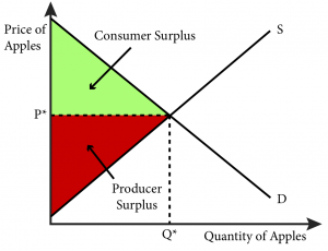
There is clearly surplus being created by the apple transactions that take place within the market. This in itself is the primary argument for the marketplace. Buyers and sellers are able to transact and become better off for it. The value to those individuals is measured by surplus.
But a complete answer must compare the value to society of the markets to the cost to society of the marketplace itself. Does the total surplus created by the marketplace justify the cost?
Let’s return now to the key assumption – that a market for fresh apples would not exist without government support. Is this a reasonable assumption?
In the 19th and early 20th centuries when many public markets were founded, transportation was difficult and bringing fresh food to support urban population centers was something local governments commonly did. Today, transportation is not nearly as difficult or costly. But although many areas are well served by grocery stores, where it is reasonable to expect customers will find fresh fruits and vegetables, other locations are characterized by food deserts:
Food deserts are defined as urban neighbourhoods and rural towns without ready access to fresh, healthy, and affordable food. Instead of supermarkets and grocery stores, these communities may have no food access or are served only by fast food restaurants and convenience stores that offer few healthy, affordable food options. The lack of access contributes to a poor diet and can lead to higher levels of obesity and other diet-related diseases, such as diabetes and heart disease. (U.S. Department of Agriculture (USDA))
The USDA estimates that 23.5 million people in the United States live in food deserts.
Although the Capitol Hill neighbourhood experienced some hard times in the past, today it is prosperous and well served by grocery stores. So the need for government support of the Eastern Market there is less clear. In Section 7 we will explore public goods and externalities in detail and become better equipped to fully explore this issue.
Exploring the Policy Question
- What other kinds of marketplaces can you think of that the government aids by providing infrastructure?
- Airports allow the market for airline travel to exist in a functional way. Most airports in the United States are run by local governments. Using the topics explored in this module, give a justification for government expenditures on airports.
- Should the District of Columbia government spend money on a market that primarily serves one neighbourhood? Give reasons for and against.
Candela Citations
- Authored by: Joel Bruneau & Clinton Mahoney. License: CC BY-NC-SA: Attribution-NonCommercial-ShareAlike
- Module 10: Market Equilibrium u2013 Supply and Demand. Authored by: Patrick Emerson. Retrieved from: https://open.oregonstate.education/intermediatemicroeconomics/chapter/module-10/. License: Public Domain: No Known Copyright
- Demand and Consumer Surplus. Authored by: Preston McAfee & Tracy R Lewis. Retrieved from: https://resources.saylor.org/wwwresources/archived/site/textbooks/Introduction%20to%20Economic%20Analysis.pdf. License: CC BY-NC-SA: Attribution-NonCommercial-ShareAlike
- Supply and Profit. Authored by: Preston McAfee & Tracy R Lewis. Retrieved from: https://resources.saylor.org/wwwresources/archived/site/textbooks/Introduction%20to%20Economic%20Analysis.pdf. License: CC BY-NC-SA: Attribution-NonCommercial-ShareAlike
- Market Demand and Supply. Authored by: Preston McAfee & Tracy R Lewis. Retrieved from: https://resources.saylor.org/wwwresources/archived/site/textbooks/Introduction%20to%20Economic%20Analysis.pdf. License: CC BY-NC-SA: Attribution-NonCommercial-ShareAlike
- Equilibrium. Authored by: Preston McAfee & Tracy R Lewis. Retrieved from: https://resources.saylor.org/wwwresources/archived/site/textbooks/Introduction%20to%20Economic%20Analysis.pdf. License: CC BY-NC-SA: Attribution-NonCommercial-ShareAlike
is the condition where the quantity supplied by producers and the quantity demanded by consumers are equal
the price at which quantity demanded equals the quantity supplied
is the the demand curve expressed with price as a function of quantity
the supply curve expressed with price as a function of quantity
the quantity at which supply equals demand
occurs when, at a given price, firms supply more of a good than consumers demand
occurs when, at a given price, consumers demand more of a good than firms supply
refers to the economic well-being of society as a whole, including producers and consumers
the difference between the price received and the willingness-to-accept price
the difference between the willingness-to-pay price and the price paid
the sum of producer surplus and consumer surplus
describes an allocation of goods and services in which no redistribution can occur without making someone worse off
the loss of total surplus that occurs when there is an inefficient allocation of resources
