Module 16: Models of Oligopoly – Cournot, Bertrand and Stackleberg

Policy Example: How Should the Government Have Responded to Big Oil Company Mergers?

Exploring the Policy Question

1. What are the strategic incentives for banks to take risks?
2. What policy solutions present themselves from this analysis?

16.1 Cournot Model of Oligopoly: Quantity Setters

Learning Objective 16.1: Describe game theory and they types of situations it describes.

16.2 Bertrand Model of Oligopoly: Price Setters

Learning Objective 16.2: Describe normal form games and identify optimal strategies and equilibrium outcomes in such games.

16.3 Stackelberg Model of Oligopoly: First Mover Advantage

Learning Objective 16.3: Describe sequential move games and explain how they are solved.

 

16.1 Cournot Model of Oligopoly: Quantity Setters

Learning Objective 16.1: Describe game theory and they types of situations it describes.

Oligopoly markets are markets in which only a few firms compete, where firms produce homogeneous or differentiated products and where barriers to entry exist that may be natural or constructed. There are three main models of oligopoly markets, each consider a slightly different competitive environment. The Cournot model considers firms that make an identical product and make output decisions simultaneously. The Bertrand model considers firms that make and identical product but compete on price and make their pricing decisions simultaneously. The Stackelberg model considers quantity setting firms with an identical product that make output decisions simultaneously. This module considers all three in order beginning with the Cournot model.

Table 16.1: Metrics of the Four Basic Market Structures

	Number of Firms	Similarity of Goods	Barriers to Entry or Exit	Module
Perfect Competition	Many	Identical	No	13
Monopolistic Competition	Many	Distinct	No	19
Oligopoly	Few	Identical or Distinct	Yes	18
Monopoly	One	Unique	Yes	15

Oligopolists face downward sloping demand curves which means that price is a function of the total quantity produced which, in turn, implies that one firm’s output affects not only the price it receives for its output but the price its competitors receive as well. This creates a strategic environment where one firm’s profit maximizing output level is a function of their competitors’ output levels. The model we use to analyze this is one first introduced by French economist and mathematician Antoine Augustin Cournot in 1838. Interestingly, the solution to the Cournot model is the same as the more general Nash equilibrium concept introduced by John Nash in 1949 and the one used to solve for equilibrium in non-cooperative games in Module 17.

We will start by considering the simplest situation: only two companies who make an identical product and who have the same cost function. Later we will explore what happens when we relax those assumptions and allow more firms, differentiated products and different cost functions.

Let’s begin by considering a situation where there are two oil refineries located in the Denver, Colorado area who are the only two providers of gasoline for the Rocky Mountain regional wholesale market. We’ll call them Federal Gas and National Gas. The gas they produce is identical and they each decide independently, and without knowing the other’s choice, the quantity of gas to produce for the week at the beginning of each week. We will call Federal’s output choice q_F and National’s output choice q_N , where q represents liters of gasoline. The weekly demand for wholesale gas in the Rocky Mountain region is P=A – BQ, where Q is the total quantity of gas supplied by the two firms or, Q=q_F+q_N. Immediately you can see the strategic component: the price the both receive for their gas is a function of each company’s output. We will assume that each liter of gas produced costs the company c, or that c is the marginal cost of producing a liter of gas for both companies and that there are no fixed costs.

With these assumptions in place, we can express Federal’s profit function:

Substituting the inverse demand curve we arrive at the expression

Substituting Q=q_A+q_B yields

The expression for National is symmetric:

Note that we have now described a game complete with players, Federal and National, strategies, q_F and q_N, and payoffs π_F and π_N. Now the task is to search for equilibrium of the game. To do so we have to begin with a best response function. In this case the best response is the firm’s profit maximizing output. This will depend on both the firm’s own output and the competing firm’s output.

CALCULUS APPENDIX

If the profit function is

[latex]\color{green} \frac{\partial \pi_F}{\partial q_F}=0[/latex]

If π_F = q_F ( A – B ( q_F + q_N ) -c ) then we can expand to find

Taking the partial derivative of this expression with respect to q_F

[latex]\color{green}\frac{\partial \pi_F}{\partial q_F}=A-2Bq_F-Bq_N-c=0[/latex]

If we re-arrange this we can see that this is simply an expression of MR=MC.

[latex]\color{green}A-2Bq_F-Bq_N=c[/latex]

The marginal revenue looks the same as a monopolist’s MR function but with one additional term, -Bq_N.

Solving for q_F yields:

[latex]\color{green}q_F=\frac{A-Bq_N-c}{2B}[/latex]

or

[latex]\color{green} q^*_F=\frac{A-c}{2B}-\frac{1}{2}qN[/latex]

This is Federal Oil’s best response function, their profit maximizing output level given the output choice of their rivals. It is the same best response function as the ones in Module 17. By symmetry, National Oil has an identical best response function:

[latex]\color{green} q^*_N=\frac{A-c}{2B}-\frac{1}{2}qF[/latex]

We know from Module 14 that the monopolists marginal revenue curve when facing an inverse demand curve P=A-BQ

is MR(q)=A-2Bq. It runs out in this duopolist example that the firms’ marginal revenue curves include one extra term:

The profit-maximizing rule tells us that to find profit maximizing output we must set the marginal revenue to the marginal cost and solve. Doing so yields [latex]q^*_F=\frac{A-c}{2B}-\frac{1}{2}qN[/latex] for Federal Oil, and [latex]q^*_N=\frac{A-c}{2B}-\frac{1}{2}qF[/latex] for National Oil. These are the firms’ best response functions; their profit maximizing output levels given the output choice of their rivals.

Now that we know the best response functions solving for equilibrium in the model is relatively straightforward. We can begin by graphing the best response functions. These graphical illustrations of the best response functions are called reaction curves. A Nash equilibrium is a correspondence of best response functions which is the same as a crossing of the reaction curves.

Figure 16.1.1: Nash Equilibrium in the Cournot Duopoly Model

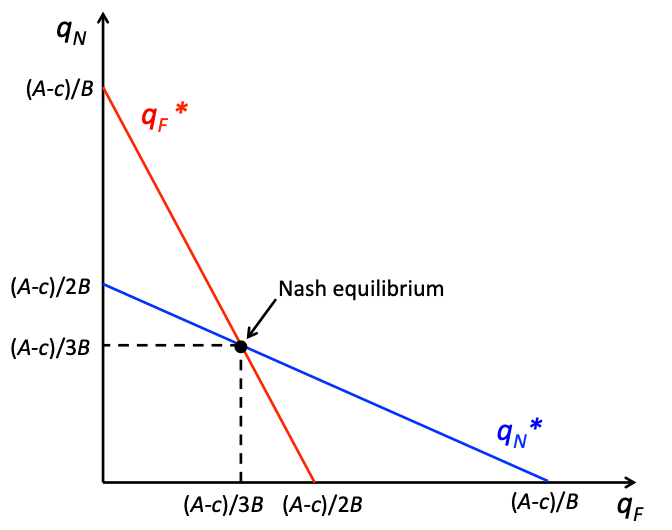
In Figure 16.1.1, we can see the Nash equilibrium of the Cournot duopoly model as the intersection of the reaction curves. Mathematically this intersection is found by solving the system of equations,  [latex]q^*_F=\frac{A-c}{2B}-\frac{1}{2}q_N[/latex] and [latex]q^*_F=\frac{A-c}{2B}-\frac{1}{2}q_F[/latex]

simultaneously. This is a system of two equations and two unknowns and therefore has a unique solution as long as the slopes are not equal. We can solve these by substituting one equation into the other which yields a single equation with a single unknown:

[latex]q^*_F=\frac{A-c}{2B}-\frac{1}{2}[\frac{A-c}{2B}-\frac{1}{2}q_F][/latex]

Solving by steps:

[latex]q^*_F=\frac{A-c}{2B}-\frac{A-c}{4B}+\frac{1}{4}q_F[/latex]

[latex]\frac{3}{4}q^*_F=\frac{A-c}{4B}[/latex]

[latex]q^*_F=\frac{A-c}{3B}[/latex]

And by symmetry we know:

[latex]q^*_N=\frac{A-c}{3B}[/latex]

The Nash equilibrium is: [latex](q^*_F,q^*_N)[/latex] , or [latex](\frac{A-c}{3B} , \frac{A-c}{3B})[/latex]

Let’s consider a specific example. Suppose in the above example the weekly demand curve for wholesale gas in the Rocky Mountain region is p = 1,000 – 2Q, in thousands of gallons, and both firm’s have constant marginal costs of 400. In this case A = 1,000, B = 2 and c = 400. So [latex]q^*_F=\frac{A-c}{3B}=\frac{1,000-400}{(3)(2)}=\frac{600}{6}=100[/latex]. By symmetry we know $latex q^*_N=100$ as well. So both Federal Oil and National Oil produce 100 thousand gallons of gasoline a week. Total output is the sum of the two and is 200 thousands gallons. The price is p = 1,000 – 2(200) = $600 for one thousand gallons of gas or $0.60 a gallon.

To analyze this from the beginning we can set up the total revenue function for Federal Oil:

[latex]TR(q_F)=p×q_F[/latex]

[latex]=(1,000-2Q)q_F[/latex]

[latex]=(1,000-2q_F-2q_N)q_F[/latex]

[latex]= 1,000-2q \frac{2}{F}-2q_Fq_N[/latex]

The marginal revenue function that is associated with this is:

[latex]MR(q_F)=1,000-4q_F-2q_N[/latex]

We know marginal cost is 400, so setting marginal revenue equal to marginal cost results in the following expression:

[latex]1,000-4q_F-2q_N=400[/latex]

Solving for [latex]q_F[/latex]:

[latex]q_F=\frac{600-2q_N}{4}[/latex]

[latex]q^*_F=150-\frac{q_F}{2}[/latex]

This is the best response function for Federal Oil. By symmetry we know that National Oil has the same best response function:

[latex]q^*_N=150-\frac{q_F}{2}[/latex]

Solving for the Nash equilibrium:

[latex]q^*_N=150-\frac{q_F}{2}[/latex]

[latex]q^*_F=150-75+\frac{q_F}{4}[/latex]

[latex]\frac{3}{4}q^*_F=25[/latex]

[latex]q^*_F=100[/latex]

We can insert the solution for [latex]q_F[/latex] into [latex]q^*_N[/latex]:

16.2 Bertrand Model of Oligopoly: Price Setters

Learning Objective 16.2:.

In the previous section we studied oligopolists that make an identical good and who compete by setting quantities. The example we used in that section was wholesale gasoline where the market sets a price that equates supply and demand and the strategic decision of the refiners was how much oil to refine into gasoline. In this section we turn our attention to a different situation in which the oligopolists compete on price. The example here are the retail gas stations that bought the wholesale gas from the refiners and are now ready to sell it to consumers. We still have identical goods, for consumers the gas that goes into their cars is all the same and we will assume away any other differences like cleaner stations or the presence of a mini-mart.

Lets imagine a simple situation where there two gas stations, Fast Gas and Speedy Gas on either side of a busy main street. Both stations have large signs that display the gas prices that each station is offering for the day. Consumers are assumed to be indifferent about the gas or the stations, so they will go to the station that is offering the lower price. So an individual gas station’s demand is conditional on its relative price with the other station

Formally we can express this with the following demand function for Fast Gas:

[latex]Q_F \left\{\begin{matrix} & & & \\ a-bP_F\,\,if\,\,P_F< P_S & & & \\ \frac{a-bP}{2}\,\,ifP_F=P_S & & & \\0 \,\,if\,\,P_S> P_F \end{matrix}\right.[/latex]

Speedy Gas has an equivalent demand curve:

[latex]Q_S \left\{\begin{matrix} & & & \\ a-bP_S\,\,if\,\,P_S< P_F & & & \\ \frac{a-bP}{2}\,\,ifP_S=P_F & & & \\0 \,\,if\,\,P_S> P_F \end{matrix}\right.[/latex]

In words, these demand curves say that if a station has a lower price than the other, they will get all of the demand at that price and the other station will get no demand. If they have the same price, then each will get one half of the demand at that price.

Let’s assume that Fast Gas and Speedy Gas both have the same constant marginal cost of c, and will assume no fixed costs to keep the analysis simple. The question we now have to answer is what are the best response functions for the two stations? Remember that best response functions are one player’s optimal strategy choice given the strategy choice of the other player. So what is one Fast Gas’s best response to the Speedy Gas’s price?

If Speedy Gas chargesP_S > c , Fast Gas can set P_F > P_S and they will get no customers at all and make a profit of zero. They could instead set P_F=P_S and get ½ the demand at that price and make a positive profit. Or they could set P_F = P_S – $0.01 , or set their price one cent below Speedy Gas’s price and get all of the customers at a price that is one cent below the price at which they would get ½ the demand. Clearly, this third option is the one that yields the most profit. Now we just have to consider the case where P_S = c. In this case, undercutting the price by one cent is not optimal because Fast Gas would get all of the demand but would lose money on every gallon of gas sold yielding negative profits. Setting P_F = P_S = c would give them half the demand at a break-even price and would yield exactly zero profits.

The best response function we just described for Fast Gas is the same best response function for Speedy Gas. So where is the correspondence of best response functions? As long as the prices are above c there is always an incentive for both stations to undercut each other’s price, so there is no equilibrium. But at P_F = P_S = c both stations are playing their best response to each other simultaneously. So the unique Nash equilibrium to this game is P_F = P_S = c.

What is particularly interesting about this is the fact that this is the same outcome that would have occurred if they were in a perfectly competitive market because competition would have driven prices down to marginal cost. So in a situation where competition is based on price and the good is relatively homogeneous, as few as two firms can drive the market to an efficient outcome.

 

16.3 Stackelberg Model of Oligopoly: First Mover Advantage

Learning Objective 16.3:

Both the Cournot model and the Bertrand model assume simultaneous move games. This makes sense when one firm has to make a strategic decision before knowing about the strategy choice of the other firm. But not all situations are like this, what happens when one firm makes its strategic decision first and the other firm chooses second? This is the situation described by the Stackelberg model where the firms are quantity setters selling homogenous goods.

Let’s return to the example of two oil companies: Federal Gas and National Gas. The gas they produce is identical but now they decide their output levels sequentially. We will assume that Federal Gas sets its output first and then, after observing Federal’s choice, National Gas decides on the quantity of gas they are going to produce for the week. We will again call Federal’s output choice q_F and National’s output choice q_N , where q represents liters of gasoline. The weekly demand for wholesale gas is still P = A – BQ , where Q is the total quantity of gas supplied by the two firms or, Q=q_F+q_N.

We have now turned the previous Cournot game into a sequential game and the SPNE solution to a sequential game is found through backward induction. So we have to start at the second move of the game: National’s output choice. When National makes this decision, Federal’s output choices is already made and known to National so it is takes as given. Therefore, we can express Federal’s profit function as:

This is the same as in the Cournot example and for National the best response function is also the same. This is because in the Cournot case both firms took the other’s output as given.

[latex]q^*_N=\frac{A-c}{2B}-\frac{1}{2}q_F[/latex]

When it comes to Federal’s decision, we diverge from the Cournot model because instead of taking q_N as a given, Federal knows exactly how National will respond because they know the best response function. Federal’s profit function, [latex]\Pi _F=q_F(A-Bq_F-Bq_N-c)[/latex], can be re-written with q_N

replaced by the best response function:

[latex]\Pi _F=q_F(A-Bq_F-B(\frac{A-C}{2B}-\frac{1}{2})-c)[/latex]

We can see that Federal’s profits are determined only by their own output once we explicitly consider National’s response. Simplifying yields:

[latex]\Pi _F=q_F(\frac{A-c}{2}-B\frac{1}{2}q_F)[/latex]

CALCULUS APPENDIX

If the profit function is

[latex]\color{green}\Pi _F=q_F(\frac{A-C}{2}-B\frac{1}{2}q_F)[/latex] then we can find the optimal output level by solving for the stationary point, or solving:

[latex]\color{green}\frac{\partial \Pi _F}{\partial q_F}=0[/latex]

If [latex]\color{green}\Pi _F=q_F(\frac{A-c}{2}-B\frac{1}{2}q_F)[/latex]

then we can expand to find

[latex]\color{green}\Pi _F=q_F(\frac{A-c}{2})q_F-B\frac{1}{2}q_{F}^{2}[/latex]

Taking the partial derivative of this expression with respect to q_F

[latex]\color{green}\frac{\partial \Pi _F}{\partial q_F}=(\frac{A-c}{2})-Bq_F=0[/latex]

Solving for q_F yields:

[latex]\color{green}q_F=\frac{A-c}{2B}[/latex]

This is Federal Oil’s profit maximizing output level given that they choose first and can anticipate National’s response.

We know that the second mover’s best response is the same as in section 15.1, and the solution to the profit optimization problem above yields the following best response function for Federal Oil:

[latex]q^*_F=\frac{A-c}{2B}[/latex]

Substituting this into National’s best response function and solving:

[latex]q^*_N=\frac{A-c}{2B}-\frac{1}{2}\left [ \frac{A-c}{2B} \right ][/latex]

[latex]q^*_N=\frac{A-c}{2B}-\left [\frac{A-c}{4B} \right][/latex]

[latex]q^*_N=\frac{A-c}{4B}[/latex]

The Subgame Perfect Nash Equilibrium is ( [latex]q^*_F[/latex] , [latex]q^*_F[/latex]).  A few things are worth noting when comparing this outcome to the Nash Equilibrium outcome of the Cournot game in section 15.1. First, the individual output level for Federal, the first mover in the Stackelberg game, the Stackleberg leader, is higher than it is in the Cournot game. Second, the individual output level for National, the second mover in the Stackelberg game, the Stackleberg follower, is lower than it is in the Cournot game. Third, the total output is larger in the Stackelberg outcome than in the Cournot outcome. This means the price is lower because the demand curve is downward sloping. Since the Cournot outcome is one of the options for the Stackleberg leader – if it chooses the same output as in the Cournot case the follower will as well – it must be true that profits are higher for the Stackelberg leader. And since both the quantity produced and the price received are lower for the Stackelberg follower compared to the Cournot outcome, the profits must be lower as well.

So from this we see the major differences in the Stackleberg model compared to the Cournot model. There is a considerable first-mover advantage. By being able to set its quantity first, Federal Oil is able to gain a larger share of the market for itself and even though it leads to a lower price, it makes up for that lower price with the increase in quantity to achieve higher profits. The opposite is true for the second mover, by being forced to choose after the leader has set its output, the follower is forced to accept a lower price and lower output. From the consumer’s perspective, the Stackelberg outcome is preferable because overall there is more quantity at a lower price.

 

SUMMARY

Review: Topics and Related Learning Outcomes

16.1 Cournot Model of Oligopoly: Quantity Setters

Learning Objective 16.1: Describe game theory and they types of situations it describes.

16.2 Bertrand Model of Oligopoly: Price Setters

Learning Objective 16.2: Describe normal form games and identify optimal strategies and equilibrium outcomes in such games.

16.3 Stackelberg Model of Oligopoly: First Mover Advantage

Learning Objective 16.3: Describe sequential move games and explain how they are solved.

Learn: Key Terms and Graphs

Terms

Oligopoly

Reaction Curves

First-Mover Advantage

Graph

Nash Equilibrium in the Cournot Duopoly Model

Table

Metrics of the Four Basic Market Structures