
19
Joel Bruneau and Clinton Mahoney
Learning Objectives
- Explain how changes in input markets affect firms’ cost of production
- Describe how individuals make their labour supply decisions and how this can lead to a backward bending labour supply curve
- Explain how monopsonist labour markets differ from competitive labour markets
- Show the labour market and welfare effects of minimum wages in a comparative statics analysis
Module 19: Input Markets
The Policy Question: Should the States of Oregon and New Jersey Prohibit Self-Service Gas?
Only two states in the United States do not allow self-service gas stations: In Oregon and New Jersey, customers are not permitted to pump their own gas. Originally, this policy was driven by safety concerns–gasoline was considered a hazardous substance due to its flammability and the adverse health effects of touching it or inhaling fumes. However, advances in pump technology have made the self-pumping of gas safe enough that 48 states and the District of Columbia have allowed self-service gas for decades. Efforts to repeal the prohibition in Oregon and New Jersey have failed and one of the key arguments from groups that defend the policy is that the repeal would lead to job losses. Economists often claim that policies that mandate employment are inefficient and cause a drag on the economy itself.
In this module we will look at input markets and study labour markets in particular. Labour is an input in retail gas, so we will be able to study this policy in depth and think about the economic implications. We can also use what we have learned so far about product markets to think through the implications for consumers.
Exploring the Policy Question
- Do you think prohibiting self-service gas is a good policy? Why or why not?
- Do you think that policies such as this one help ensure that there is adequate employment?
19.1 Input Markets
Learning Objective 19.1: Explain how changes in input markets affect firms’ cost of production.
19.2 Labour Markets
Learning Objective 19.2: Describe how individuals make their labour supply decisions and how this can lead to a backward bending labour supply curve.
19.3 Competitive Labour Markets and Monopsonist Labour Markets
Learning Objective 19.3: Explain how monopsonist labour markets differ from competitive labour markets.
19.4 Minimum Wages and Unions
Learning Objective 19.4: Show the labour market and welfare effects of minimum wages in a comparative statics analysis.
19.1 Input Markets and Employment
LO 19.1: Explain how changes in input markets affect firms’ cost of production.
In Module 7, we learned that when firms produce a good or service they do so by combining various inputs. These inputs, also known as factors of production, have a price. For example we learned that capital has a price called the rental rate and labour has a price called the wage. But inputs can be almost anything, like aluminum for auto manufacturers, cocoa beans for chocolate makers, or fresh produce for a restaurant. When firms buy these inputs they do so on goods markets and act as consumers just like those in our demand models. In that way input markets are just the same as the markets we have already studied. In most cases, the markets work like the goods markets we have studied, but there are some important exceptions, and we will study two in this module.
The first exception comes from the input used by virtually every producer, labour. Labour markets have particular features that make them different than normal product markets. The first is that labour is not a good or service supplied by a firm but the physical and mental effort exerted by individuals in exchange for a wage. There are both physical constraints on the supply of labour–a person cannot supply more than 24 hours worth in a day–and constraints that come from individuals’ decisions to consume leisure time as well as tangible goods and services.
The second exception comes from the fact sometimes suppliers of inputs supply a single company. Thus the purchasing company acts as a monopsonist: a single buyer for goods or services sellers. Monopsony is the term used to describe a market in which there exists only one buyer for a good. Monopsonies are rare, but they do exist. Examples are the market for sophisticated weaponry for which there is only one legal buyer, the Department of Defense, and the market for labour in “company towns” where one firm employs most of the workers in the town.
Before studying the exceptions, let’s take a look at a typical input market that acts as a normal goods market, with many sellers and many buyers. Consider a company like Dell that sells PC computers fully assembled and ready to use. This company may make component parts themselves but also likely purchases component parts from other suppliers as well. Let’s suppose that Dell buys computer hard drives (HDD) from various suppliers. There are many manufacturers of computer hard drives and many potential buyers, including individuals who wish to build or upgrade their own computers, so the computer hard drive market is very typical of a standard goods market.
Note that the hard drive market is both an input market, as hard drives are inputs in the manufacture of Dell computers, and a final goods market, as hard drives are also final purchases of consumers. Some goods, like raw iron, are almost exclusively inputs because there is no demand for raw iron as a final consumer good. A good that is used as an input to produce other goods is called an intermediate good. Other goods, like a pair of denim jeans pants, are purchased by the end user. Such a good is called a final good. And some goods, like computer hard drives, are both intermediate and final goods.
Manufacturers like Dell purchase computer hard drives in product markets along with regular consumers, though they typically buy direct from the manufacturers and not through retailers, as do consumers. Regardless, the price they pay for their hard drives is set by the hard drive goods market as illustrated in Figure 19.1.1, which shows the market for one particular type of drive: the one terabyte HDD (1TB HDD).
Figure 19.1.1 The Market for One Terabyte Computer Hard Drives (1TB HDD)
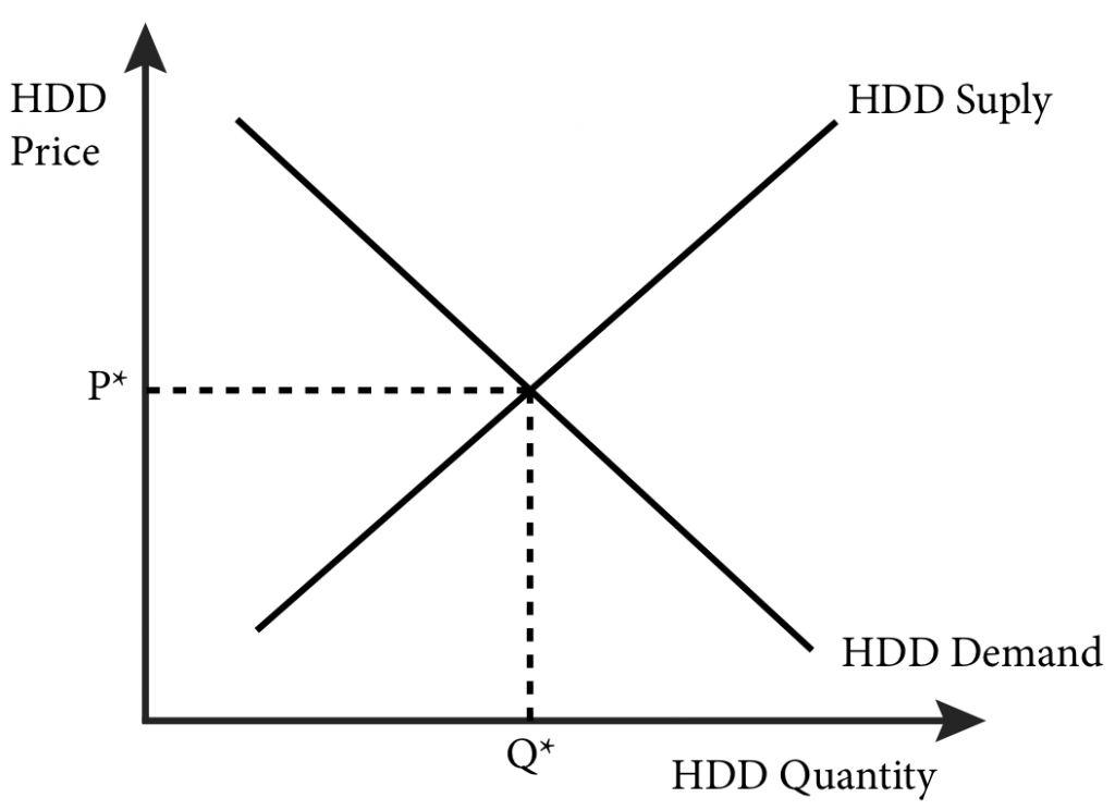
In figure 19.1.1, there are many suppliers of hard drives and many demanders. The demanders are both manufacturers and consumers. Since this is the market for wholesale 1TB HDDs, consumers are represented by retailers like Fry’s, Amazon, and New Egg. The price of a 1TB HDD is determined by the market as P*. This P* is an input price for computer manufacturers, just like the rental rate on capital, r, and the wage rate for labour, w, as we studied in Module 7. The same market dynamics of goods markets apply here: when demand or supply changes, prices will change as well. For example, if new manufacturers of 1TB HDD enter the market the price for these goods will fall. If there is a new substitute for 1TB HDD, like solid state hard drives, demand could fall, which would also lower the price of the good.
Price changes in the input markets will affect the cost conditions of firms as we saw in Module 7 and will, in turn, affect the supply of the final good. As input prices rise, the supply curve in the final good market shifts to the left and the price of the final good rises. As input prices fall, the supply curve of the final good market shifts to the right and the price of the final good falls.
As noted above, the typical behavior of input markets changes when the input is labour or when the buyer of the input is the only buyer. We study these two instances in the next two sections.
19.2 Labour Markets
LO 19.2: Describe how individuals make their labour supply decisions and how this can lead to a backward bending labour supply curve.
Almost every final good produced has some labour input involved, if not as part of the manufacturing process than as an ancillary contribution through administration, marketing, sales and so forth. For this reason alone, labour has an outsized role in production and deserves special attention. Another particular aspect of labour that requires special attention is the fact that it is an input provided by individuals making optimal decisions about work and leisure.
The labour market is where labour prices, or wages, are set and is defined by the same supply and demand dynamics as other input markets. The supply of labour is determined by the labour-leisure choice of individuals. Individuals think about the tradeoff between working more and earning more money, which can be used to purchase goods and services, and working less and having more time to enjoy leisure activities and perform chores that are necessary but for which there is no monetary compensation.
The labour-leisure choice is the starting point to thinking about labour markets. We can model this choice just as we do consumers deciding between bundles of two different goods. Both leisure and the income from labour are goods that reflect standard preferences: individuals would prefer more of both, and a mix of both income and leisure is preferable to too much of one or the other. Thus we can describe an individual’s preferences by a utility function of income (I) and leisure (l):
U = U(I , l)
Individuals cannot spend more than 24 hours per day in either activity. We can write down a constraint that describes this as:
H = 24 – l,
where H is the hours spent working in a day and l is the amount of leisure consumed in a day. For a given hourly wage rate, w, the income earned by a consumer, I, is given as:
I = wH.
Recall that in Module 4, where we studied the consumer choice problem, we took income (I) as given to the consumer. In this discussion we will see that I is a result of a decision the individual makes about how much labour to supply to the labour market.
Figure 19.2.1 shows the optimal choice between leisure and income for an individual, Asha, and how it is determined. Asha’s income is measured on the vertical axis and the amount of leisure hours per day she consumes is measured on the horizontal axis. Since there are only 24 hours in a day, Asha cannot consume more than 24 hours of leisure. Note that the less leisure she consumes, the more time she spends on labour and the more income she earns.
Figure 19.2.1 shows Asha’s budget constraint line in black. If the wage rate is w1, the budget constraint has the slope of −w1. This is because for every extra hour of leisure she consumes, she loses w1 in income. The highest indifference curve Asha can achieve is given as U1 and is shown in red. Maximizing her utility at the wage rate of w1 yields a choice of I1 in income and l1 in leisure.
Figure 19.2.1 The Optimal Labour–Leisure Choice Problem
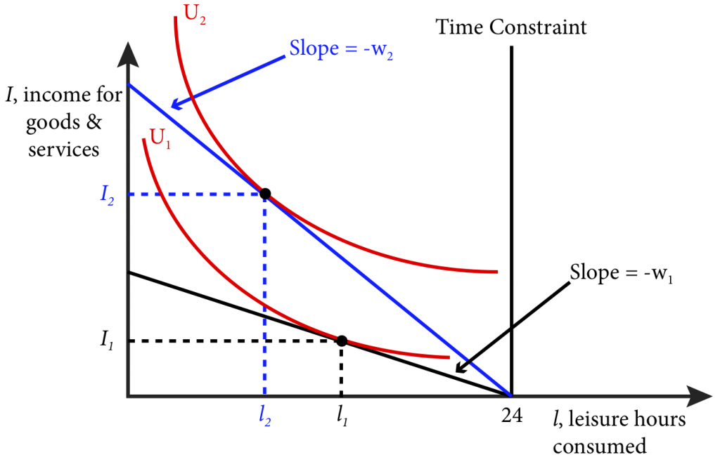
Now what happens when the wage rate increases to w2? Asha’s new budget constraint, shown in blue, lies above the old budget constraint. This is because at a higher wage, Asha gets more income for every hour spent working or not consuming leisure. The highest indifference curve she can achieve at this budget constraint is given as U2. How does Asha adjust her consumption? Since the opportunity cost of leisure has increased, she gives up more income when she consumes leisure and she consumes less leisure. Maximizing her utility at the wage rate of w2 yields a choice of I2 in income and l2 in leisure.
From the solutions to this optimal labour-leisure choice problem we can derive the demand curve for leisure for Asha (Figure 19.2.2).
Figure 19.2.2 An Individual’s Leisure Demand Curve
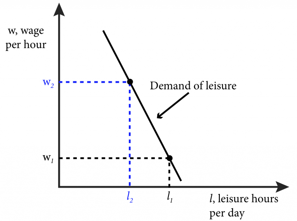
At wage w1, Asha consumes l1 hours of leisure and at wage w2, Asha consumes l1 hours of leisure. Her demand for leisure is a curve that connects these two points. Note that the wage rate is cost or price of leisure; as it increases, Asha demands less leisure. Going from Asha’s demand for leisure to her supply of labour simply requires that we subtract her leisure demand from the 24 hours available to Asha to spend on both labour and leisure, H = 24 – l, where H is the work hours per day. Figure 19.2.3 illustrates Asha’s labour supply curve.
Figure 19.2.3 An Individual’s Labour Supply Curve
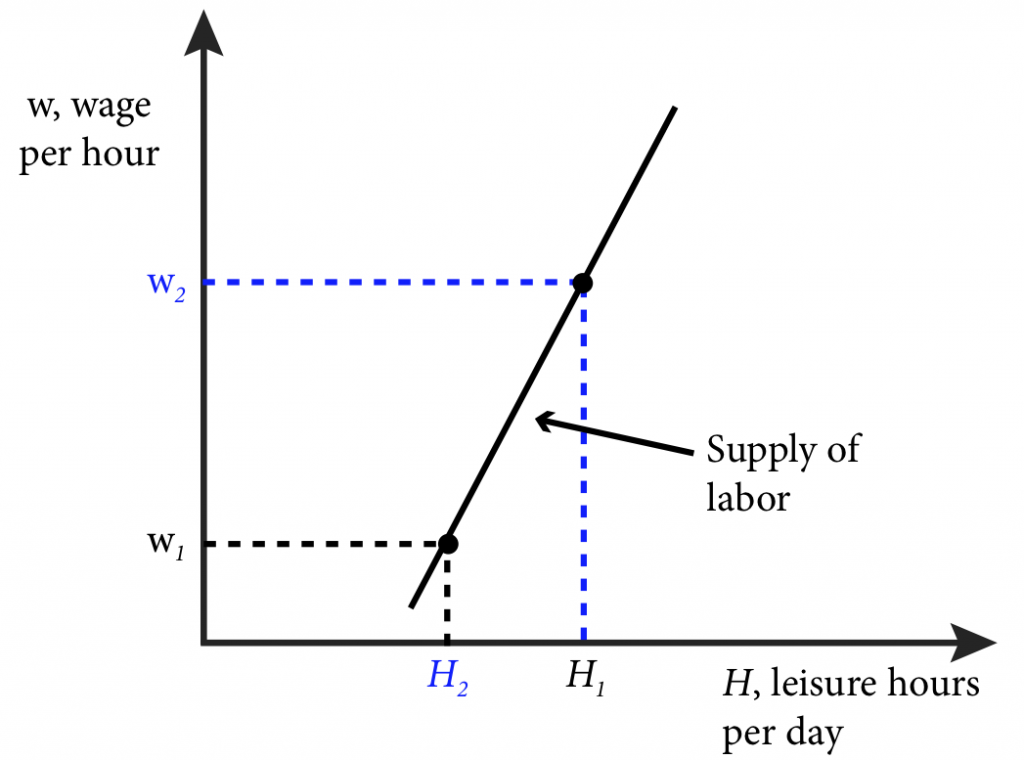
Asha’s labour supply curve, as depicted in Figure 19.2.3 is an upward sloping curve. The curve shows that the effect of an increase in the wage is an increase in hours of labour supplied from H1 to H2. This change, however, is the net effect of both the income and substitution effects, which we studied in Module 5.6. The income effect refers to the fact that as the wage rises, Asha has more money to spend on both leisure and other goods and, if the goods are both normal, she will want to consume more of both. The substitution effect refers to the fact that as the wage rises, leisure becomes more expensive relative to the consumption of other goods and Asha will naturally substitute away from leisure and toward the increased consumption of other goods as enabled by more work at the higher wage. If the substitution effect dominates the income effect then her labour supply will be upward sloping as in Figure 19.2.3.
Suppose, however, that the income effect dominates the substitution effect. In this case Asha will choose to consume more leisure as wage rises and her labour supply curve will be backward bending. This might be more likely as wages rise high enough that individuals can satisfy much of their material consumption desires and increase their consumption of leisure. Put another way, there may be a point where increased income causes individuals to actually choose to work less so that they can have more time to enjoy the consumption of their goods, services and leisure. Figure 19.2.4 illustrates this situation. Panel a shows three different wages and the corresponding leisure choice for each. Panel b illustrates the resulting labour supply curve, which starts positively sloped but then bends backwards at higher wages.
Figure 19.2.4: The Backward Bending Labour Supply Curve
a) The Labour-Leisure Choice
b) Labour Supply Curve Slopes Upward at Lower Wages and then Bends Backward at Higher Wages
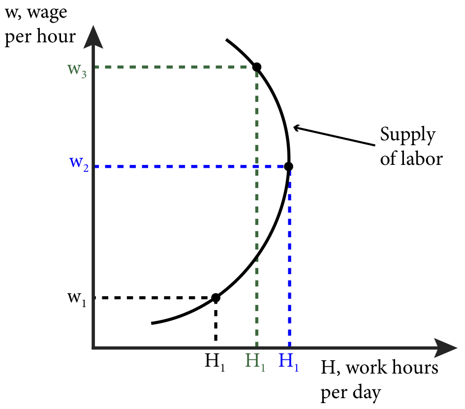
When the wage rises from w1 to w2, Asha decides to work more hours and consume less leisure. However, when wages rise from w2 to w3, Asha decides that her income is high enough that she would like to consume more leisure and work less. That is, her new wage allows her to consume more of both goods (leisure and all other goods). In this case the income effect, which causes her to want to consume more of both goods, outweighs the substitution effect, which causes her to substitute away from the relatively more expensive good, leisure, and toward the relatively less expensive good, consumption of other goods.
This analysis shows that a backward bending labour supply is theoretically possible, but do such labour supply curves actually exist? Only empirical research can answer this question. But there are some assumptions that are not quite accurate for many workers, the first being the characterization of the labour-leisure choice. Most workers cannot choose independently how many hours per day they work. Many jobs have specified work hours and in the United States, many jobs are 40 hours a week with very little room for adjustment. So when employers raise wages, there may be no way for employees to adjust their hours in response. Empirical research suggests that for men this rigidity in hours might be very important as their labour supply curves have been estimated to be nearly vertical.
19.3 Competitive Labour Markets and Monopsonist Labour Markets
LO 19.3: Explain how monopsonist labour markets differ from competitive labour markets.
Another way that input markets can be different than a typical goods market is when there is only one buyer of an input. Monopsony is the situation where there are many sellers but only one buyer of a good. Consider the case of an advanced weapon system that by law can only be sold to the government, or a factory town where almost all of the resident workers are employed by a single factory.
The case of professional American football players in the United States is a good example. The National Football League (NFL) is the only major professional American football league in the world, and while there are a few other options, like the Canadian Football League, they pale in comparison to the NFL. In labour market terms the NFL acts a lot like a single entity with strict rules about hiring that prevent teams from competing with each other for new talent. Each year there are many sellers of labour, the football players, and one buyer, the NFL.
Competitive Firms’ Employment Behavior
How are monopsonists different than competitive firms in a labour market? To answer this let’s first look at competitive firms’ hiring decisions. In a competitive labour market each firm has no influence on the equilibrium market wage, so no matter how many workers or worker hours a firm employs the wage will remain constant. Thus a firm’s decision is to continue to employ workers as long as the value of their marginal product of labour (MPL) is greater than the wage. Recall that MPL, is the extra output achieved from the addition of a single unit of labour. For our discussion here the unit is an hour of work. The marginal revenue product of labour (MRPL) is the value of the marginal product of labour—it is the extra revenue a firm receives for an additional unit of labour. Therefore the MRPL is the product of the marginal product of labour and the marginal revenue, MR, that accrues to the firm from one additional unit of output:
MRPL = MR × MPL
A firm will continue to add additional hours of labour as long as that additional labour adds positively to profits. The cost of an hour of labour is w and the benefit is precisely the MRPL. So as long as MRPL > w the firm is adding to its profits. If MRPL < w, the firm can increase its profits by reducing the number of labour hours it uses. The firm maximizes its profits from its employment decisions only at the point where MRPL = w. So we can characterize the firm’s employment rule as:
MRPL = w
In a competitive output market the MR is equal to the price that each unit sells for in the market, or the market price, p. So MRPL = p × MPL. The firm’s employment rule becomes:
p × MPL = w(12.3.1)
Dividing both sides by MPL yields:
p = w/MPL
We know from Module 9 that profit-maximizing firms produce to the point where marginal revenue equals marginal cost. Marginal revenue is p as we just discussed, so the profit-maximizing rule is:
p = MC.
Putting together the employment rule and the profit maximization rule we get:
p = w/MPL = MC
Recall from Section 7.3 that as the firm adds incremental units of labour, the MPL increases up to a certain point, and then begins to fall due to inefficiency. Beyond this point, the firm must reduce units of labour in order to increase MPL. We can combine this fact with the expression of labour demand in Equation 19.3.1 to explain the firm’s employment behavior.
Specifically, with p fixed from the final goods market, as w rises, the firm will reduce worker hours in order to increase MPL and so maintain the equality in (19.3.1). We can see this in Figure 19.3.1 which shows in black the labour demand curve, D, when price is p. At wage w1 the firm will employ L1 hours of labour; when wages rise to w2 the firm will reduce employment to L2. This is a shift along the labour demand curve as wages change.
Figure 19.3.1: The Labour Demand Curve and Wage and Price Changes
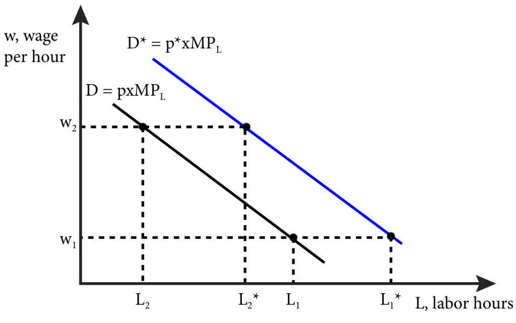
What happens when the price of the final good changes? Well suppose the price rises from p to p*. This means that the MRPL rises as well and so temporarily the p × MPL > w. The firm can now add more workers to lower the MPL until the equality of the MRPL to w is restored. We see this in Figure 19.3.1 as a shift in the labour demand curve from D (in black) to D* (in blue). Now at wage w1 the firm will employ L1* hours of labour and when wages rise to w2 the firm will reduce employment to L2*.
To summarize the results of wage and price changes on the labour demand curve:
- A change in wage results in a shift along the labour demand curve.
- A change in price results in a shift of the labour demand curve.
Wages and Labour Market Equilibrium
How is the wage amount set in a competitive labour market? To find labour market equilibrium we must first derive the market supply of labour and the market demand for labour.
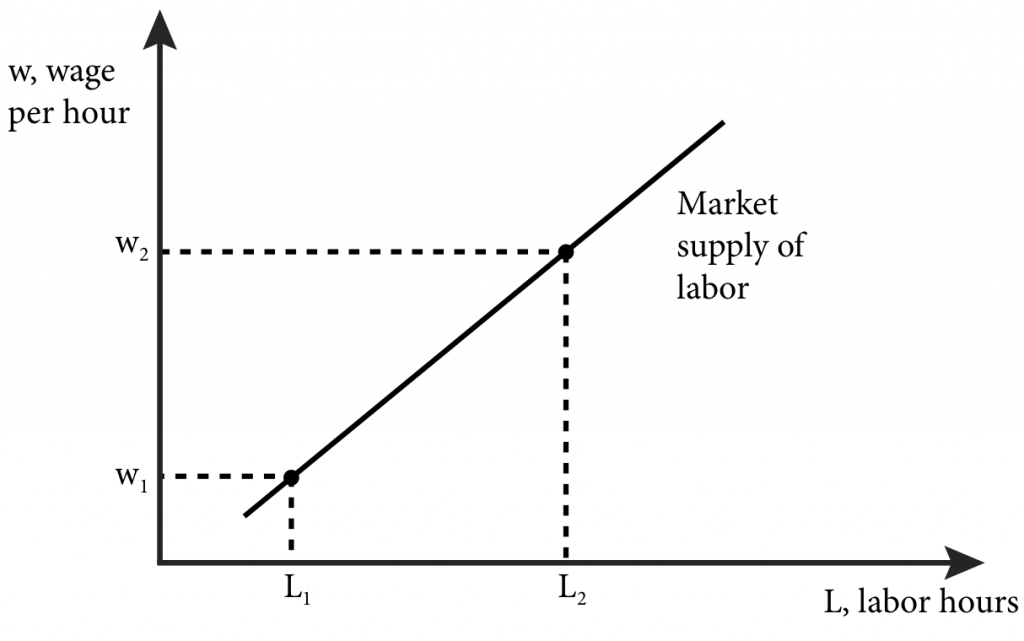
The market supply of labour is simply the sum of the labour supplied by all individual workers. Figure 19.2.3 showed an individual labour supply curve;. the market labour supply curve is illustrated in Figure 19.3.2. Labour hours, L, is simply all of the individual work hours per day, H, for every potential worker. As the wage increases, the number of workers and the number of hours each worker is willing to work increases as well and the result is an upward sloping curve.
Figure 19.3.2: The Market Supply of Labour
We find the market demand for labour by summing up the individual firms’ labour demands. Once we have the market demand for labour we can graph it together with the market supply of labour, as shown in Figure 19.3.3. Doing so reveals the labour market equilibrium, identical to the equilibrium in other goods markets, and the resulting equilibrium wage rate, w*, and total employment, L*.
Figure 19.3.3: Labour Market Equilibrium
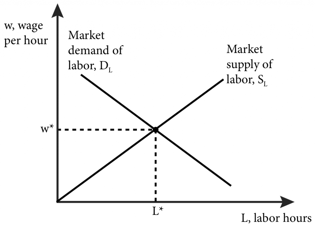
As Figure 19.3.3 shows, we call the market demand for labour DL and the market supply of labour SL. Where they cross is the equilibrium point and the wage and labour hours at that point are the equilibrium wage rate, w*, and equilibrium employment, L*, respectively.
Monopsony Employment Behavior
In a competitive labour market the wage amount is set by market equilibrium of labour supply and demand, and the firm must pay that wage in order to attract workers. But when the firm is a monopsonist in the labour market, it has power to influence the wage amount, w, and does not take it as fixed.
A competitive firm takes the wage as given and can hire as many work hours as it likes at that wage. We call the marginal expenditure (ME) the extra cost of hiring one more unit of labour. The ME for a competitive firm of an additional hour of labour is simply the market wage.
A monopsonist must also pay a wage to attract workers but this wage depends on the labour supply curve. For example, suppose that at a wage of $20 per hour, a monopsonist firm attracts 1000 hours of workers per week for a total weekly wage bill of $20,000. Now suppose the price of its product has increased and it wants to increase production. To do so, the firm will have to hire more work hours by raising the wage.
Suppose that at $25 per hour the firm now attracts 1,200 hours of workers. The firm’s total wage bill has now increased not just by the extra 200 hours of work at $25, or $5000, which would increase its wage bill to $25,000. Rather, it now pays for all of its labour hours at $25. This increases the wage bill to $30,000 (1,200 × $25). So the marginal expenditure, ME, of an additional hour of labour is not just the additional wage the firm has to pay for that hour of work but the additional wage the firm has to pay for all hours of work.
Figure 19.3.4 illustrates the marginal expenditure curve for a monopsonist firm. The ME curve lies above the market supply of labour curve because of the fact that the firm cannot pay for one additional hour of work at a slightly higher rate than the rest. It must pay the same wage for all hours of work. The firm is therefore no longer setting its MRPL equal to the wage, but to the ME. We can state this insight about labour market equilibrium in the case of a monopsonist firm as:
MRPL = ME
Figure 19.3.4: Monopsony and the Marginal Expenditure Curve
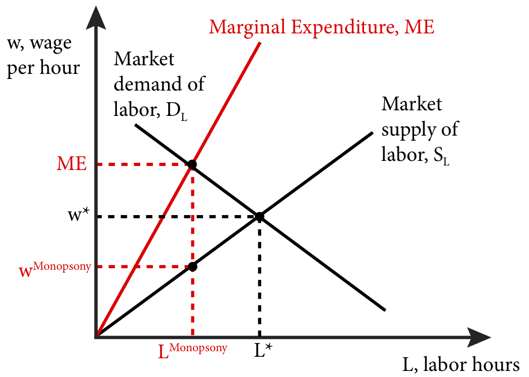
For a monopsonist firm, the MRPL curve is the labour demand curve. The firm’s optimal employment decision is where ME = DL. This occurs at LMonopsony. To attract this amount of labour the firm must pay wMonopsony – the point on the supply curve that yields precisely LMonopsony. We can see from figure 19.3.4 that the monopsonist will hire fewer hours of labour (LMonopsony) than would occur in a competitive market (L*) and pay a lower wage (wMonopsony) than in a competitive market (w*).
19.4 Minimum Wages and Unions
Learning Objective 19.4: Show the labour market and welfare effects of minimum wages in a comparative statics analysis.
In a monopsonist labour market, the buyer of labour—the firm–has some power to set wages, rather than accepting a market-driven rate. In other contexts, the sellers of labour—workers—may enjoy an advantage in determining wage rates or employment levels or both. These advantages can be achieved through collective bargaining, for example, or public policy approaches such as setting a minimum wage.
In the United States it is illegal to pay workers below the federally mandated minimum wage, currently set at $7.25 an hour. Many states have set minimum wages above this level; in 2015 Washington was the state with the highest minimum wage, at $9.47 an hour. There are many reasons for these policies but the most common rationale, often expressed by those who champion even higher minimum wages, is that wages are too low and do not represent a ‘living wage’ – a wage high enough to afford the basic necessities of food, shelter and clothing. In other words, minimum wages are a policy tool to address poverty.
To analyze minimum wages, we start by recognizing that they are price floors in the labour market. A minimum wage set above the market equilibrium wage moves the market leftward on the market demand for labour curve, as Figure 19.4.1 shows. As a result, fewer employers are able to enter or remain in the market and existing employers demand fewer hours of labour at the minimum wage than at the market equilibrium wage, w*. At the same time, more workers are interested in entering the market and existing workers are willing to work more hours at the higher minimum wage than at the market equilibrium wage. This difference between the number of hours that workers would like to work (LSupplied) and the number of labour hours that employers demand (LDemanded) leads to an excess supply of labour at the minimum wage, as shown in Figure 19.4.1 .
Figure 19.4.1: Minimum Wage in a Labour Market
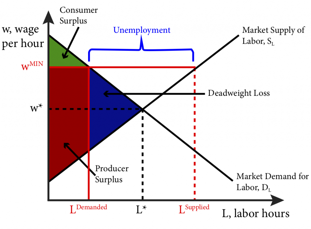
Economists describe the difference between the employment level at the equilibrium wage, L*, and the employment level at the minimum wage, LDemanded, the disemployment effect: the amount of employment lost due to the minimum wage. We refer to the difference in the amount workers would like to work at the minimum wage and the amount they actually do work as unemployment. Unemployment occurs when there are people who would like to work at a given wage but are unable to find employment.
Unions are labour groups that bargain collectively for wages for a group of workers in a company. Their objective is to leverage collective bargaining to achieve higher wages than would have occurred in the individual labour market. In this sense then we can think of the result of unions in a similar way to minimum wages set by governments: they create a price floor in labour markets.
How do wage floors affect the welfare of workers and firms? Put another way, how do wage floors affect producer surplus and consumer surplus? Remember that in the context of labour, workers are the producers and firms are the consumers.
Let’s start by looking at the producers. Those workers able to find employment at the new wage and equal in hours to what they had at the previous wage are better off because they receive higher compensation for the same work. Workers that are unable to find work at the new wage and who had work at the old wage, are worse off; they want to work, but cannot and so have no compensation. Workers who did not work prior to the minimum wage and continue not to work after it see no change in their welfare.
Producer surplus for those that have work rises. But remember the caveat from Module 12: this assumes that we are employing only those on the lowest part of the supply curve. There is no mechanism to ensure this so the producer surplus shown in Figure 19.4.1 is really a maximum possible surplus and it is likely to be substantially lower.
On the firm side, consumer surplus falls. This occurs because firms must pay more for the workers they employ and they employ fewer workers. Overall societal welfare falls unequivocally, as seen in Figure 19.4.1. The new wage creates deadweight loss, signifying a lower level of total surplus than prior to the wage floor due to the lower overall level of employment.
Studies that have looked at the impact of minimum wage laws have found different results. The broad picture appears to be that minimum wages do have a disemployment effect but that the effect tends to be quite small. The likely reason for this is the relative inelasticity of labour supply and demand curves at the bottom edge of the wage scale.
Inelastic labour demand and supply mean that the labour demanded and labour supplied are very insensitive to changes in wages. Figure 19.4.2 shows this inelasticity as very steeply sloped labour demand and supply curves. The graph shows that as wage is raised to a minimum above the competitive wage there is very little impact on labour demanded and labour supplied. As a result, the difference between the two—that is, unemployment at the minimum wage–is relatively small, as is the deadweight loss.
A final question we might ask is whether minimum wages are effective poverty fighting tools. In this case the evidence is more mixed. In the United States, relatively few of those working for minimum wages are key income earners for poor households. Many of these jobs are held by teens and young adults that work part time for some extra income and are from wealthier households. So while there seems to be a fairly limited detrimental impact associated with minimum wages, economists tend to prefer more targeted policies for fighting poverty, like the Earned Income Tax Credit (EITC), which transfers money directly to the poorest working households.
SUMMARY
Review: Topics and Related Learning Outcomes
19.1 Input Markets
Learning Objective 19.1: Explain how changes in input markets affect firms’ cost of production.
19.2 Labour Markets
Learning Objective 19.2: Describe how individuals make their labour supply decisions and how this can lead to a backward bending labour supply curve.
19.3 Monopsony
Learning Objective 19.3: Explain how monopsonist labour markets differ from competitive labour markets.
19.4 Minimum Wages and Unions
Learning Objective 19.4: Show the labour market and welfare effects of minimum wages in a comparative statics analysis.
Learn: Key Terms and Graphs
Terms
Marginal revenue product of labour (MRPL)
Graphs
The Market for One Terabyte Computer Hard Drives (1TB HDD)
The Optimal Labour–Leisure Choice Problem
An Individual’s Leisure Demand Curve
An Individual’s Labour Supply Curve
The Backward Bending Labour Supply Curve
The Labour Demand Curve and Wage and Price Changes
Monopsony and the Marginal Expenditure Curve
Minimum Wage in a Labour Market
Supplemental Resources
YouTube Videos
There are no supplemental YouTube videos for this module.
Policy Example
Policy Example: Should the Government Prohibit Self-Service Gas?
The prohibition on self-service gas in New Jersey and Oregon is, in essence, a mandate that retail gas stations employ workers who perform the task of pumping gas into cars. In the labour market for gas station workers, this policy has the effect of increasing the demand for labour. In fact, such a policy has the double effect of increasing both employment and wages as shown in Figure 1.
Figure 1: Effect on Wages and Labour Hours of a Ban on Self-Service Gas
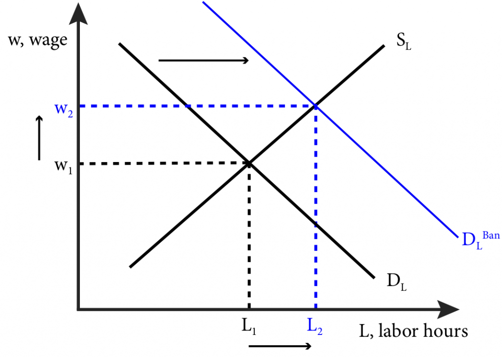
To analyze our policy question, let’s suppose that a state that does not currently have a ban on self-service gas imposes one. The resulting change in the demand for labour is the blue curve in Figure 1.
Here we see that employment in the form of labour hours increases from L1 to L2 and wages increase from w1 to w2. If this was the end of the story we might be tempted to conclude that the ban on self-service gasoline is unequivocally good.
However, we now have enough economic analysis tools to understand that labour is an input in the production of retail gas and when the cost of this input increases, the supply curve of retail gas shifts up, as Figure 2 shows. The increase in the cost of the labour input is due not only to the increased wage but also to the increased amount of labour required to pump gas. The increased cost of supplying a gallon of gas will cause retailers to supply less, shifting the supply curve leftward from S to SBan.
Figure 2: The Effect on Retail Gas Supply of a Ban on Self-Service Gas
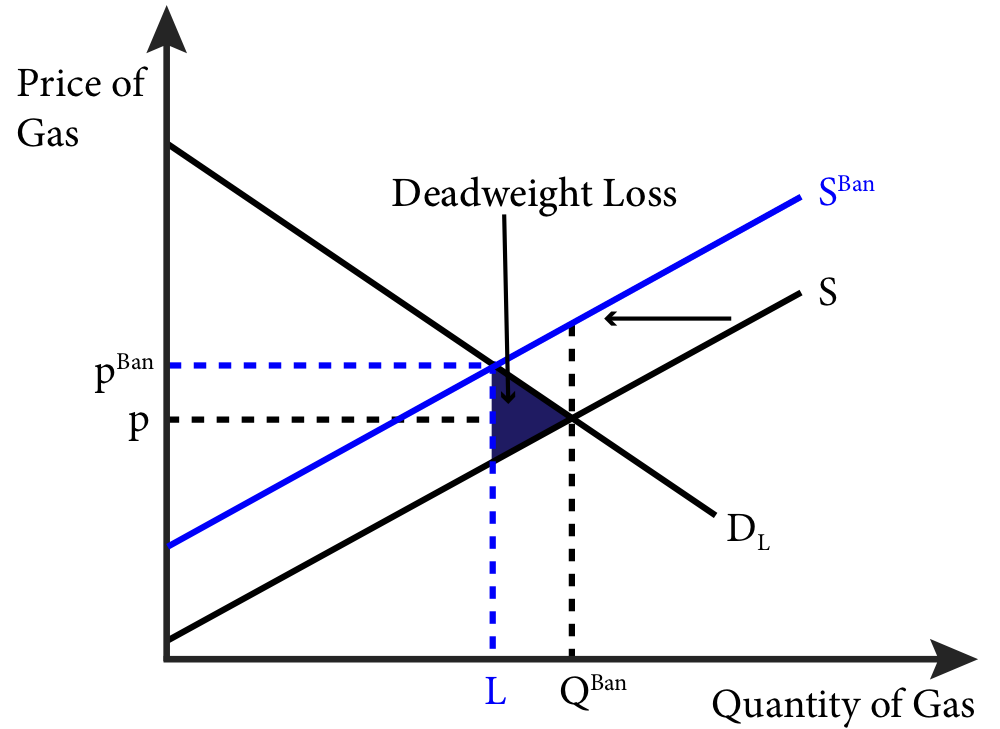
The leftward supply shift has the effect of increasing the price of gas to consumers and decreasing the amount they purchase, leading to deadweight loss. The policy question becomes, how big is this deadweight loss to society compared to the benefit to society of the increased employment among gas station attendants.
We can gain some insight into this question by comparing the states of Oregon and Washington. Oregon prohibits self-service gas while its neighbour, Washington, does not. According to the US Energy Administration (http://www.eia.gov/dnav/pet/pet_cons_prim_dcu_SWA_a.htm), in 2010 Washington had roughly twice the population of Oregon but almost identical gas consumption per capita of 400 gallons per year. Additionally, Oregon employed roughly 3.5 more people per gas station than did Washington and there were fewer stations per capita in Oregon. Extrapolating from the difference in employment, economists have estimated that the additional cost from the ban adds roughly 5 cents to the price of a gallon of gas in Oregon compared to Washington. Given that the number of extra attendants in Oregon appears to be in the vicinity of 3,000 and the population of Oregon is about 4 million, it is likely that the deadweight loss that comes from the higher price of retail gasoline is quite large relative to the societal benefit of the relatively few added employees.
Exploring the Policy Question
- Do you support the ban on self-service gas? Why or why not?
- Suppose the government mandated that grocery stores must have employees carry customers’ groceries of to their cars. What effect would be on prices and employment would you expect?
Candela Citations
- Authored by: Joel Bruneau & Clinton Mahoney. License: CC BY-NC-SA: Attribution-NonCommercial-ShareAlike
- Module 12: Input Markets. Authored by: Patrick Emerson. Retrieved from: https://open.oregonstate.education/intermediatemicroeconomics/chapter/module-12/. License: CC BY-NC-SA: Attribution-NonCommercial-ShareAlike
a single buyer for goods or services sellers
is the term used to describe a market in which there exists only one buyer for a good
a good that is used as an input to produce other goods
goods that are purchased by the end user
is the value of the marginal product of labour; it is the extra revenue a firm receives for an additional unit of labour
is the extra cost of hiring one more unit of labour or other input unit
the amount of employment lost due to the minimum wage
occurs when there are people who would like to work at a given wage but are unable to find employment
