
Appendix A: Technical Appendices
18
Module 0: introduction to imaging: two-color double stars
Learning Objectives
By the end of this module the successful student will be able to:
- request 3-filter images using Skynet telescopes
- manipulate the images in AfterGlow to produce color images
Contents
1. Purpose
2. How to request observations
3. How to make color images
4. Blog entry
5. Trouble shooting
Appendix: target list
1. Purpose
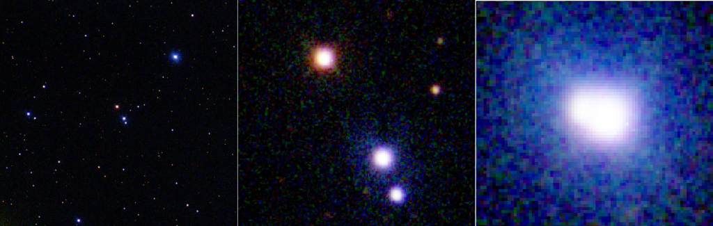
This module is optional. This module can be completed in about an hour spread over 2 or 3 days. It is designed to give a quick preview of some of the skills needed for the other imaging modules in MWU. Two-color double stars are attractive targets, and you have to concern yourself with only two things: the stars themselves, and the sky background.
Some background: Double stars are stars that appear close together on the sky from our view on Earth. If the stars are not in fact close together but instead only appear along the same line of sight then they are called optical doubles. If the stars are gravitationally bound then they are called binary stars. All the targets in this module are called visual binaries, meaning that each star in the pair can be seen separately from the other.
2. How to request observations
What follows is a recipe. More complete information is in the technical document, “Optical observing guide for Skynet”. Check with your instructor for any changes to be made to the following procedure.
- From the appendix below, choose a two-color double and note its target name.
- Log in to Skynet.
- Select “Add new observation”.
- Enter the target name in the keyword box and select “search”.
- Check that the target is visible for an appreciable fraction of the night.
- Generally the default settings are ok. Make any changes you see fit.
- Under advanced settings select “Enable dithering”. A 3-by-3 grid with 4-arcsecond spacing will do.
- Select “Save and choose filters”.
- Select Johnson-Cousins B, V, and R filters. Select “Save and continue”.
- Select all telescopes available to you. Select “Save and continue”.
- Select “Generic 16-inch” exposure efficiency.
- Filter = B. #exps = 10. Duration = 6.
- Filter = V. #exps = 10. Duration = 2.
- Filter = R. #exps = 10. Duration = 2.
- Select the appropriate time account.
- In “Advanced options” select “All exposures on same telescope”. Select “Save and continue”.
- Check all the entries on the Review page and make any changes. Select “Submit”.
- Your observations will take a day or two to come in. When they are completed then go to the next section.
3. How to make color images
Aligning and stacking
- Log in to AfterGlow.
- Select the folder icon to open your observing queue: Files – Skynet Robotic Telescope Network – User Observations – <observation name> – Reduced Images. Select all.
- Use the “filter images” box to list only the images you just imported.
- Take a quick look at every one of your 30 images. Remove any that are obviously bad; even a single bad image can ruin 100 good images during later processing.
- From the left side menu, enter any pixel operations needed; ask your instructor.
- Select the “Show WCS calibration” menu. Select all images. Select “Extract values from current viewer”. Select “Submit”. Wait for the process to finish.
- Select the “Show aligner” menu. Select all images. Select a reference image. Select “Submit”. Wait for the process to finish.
- Select the “Show stacker” menu. Select ONLY the B filter images.
- Mode = average
- Percentile = 50
- Low = 1
- High = 1
- Rejection = Chauvenet
- Scaling = Average
- Select “Submit”. Wait for the process to finish.
- Perform the previous step for ONLY the V filter images. Then perform the previous step for ONLY the R filter images.
Grouping and colorizing
- You now have three new images in your list, each with the code “_stack” in their names. On the left list, hover over the name and then select the check box for each of these three images. All three will be checked.
- At top left, select the three vertical dots, and select “Group selected files”. A new entry will appear in your file list with the three “_stack” files under the entry. Look at each of the three for any obvious errors.
- Right-click the B filter image, choose Color map – Blue.
- Right-click the V filter image, choose Color map – Green.
- Right-click the R filter image, choose Color map – Red.
- Now select the main entry. Again go to the right side and select the “Show display” icon.
- From the display page, select “Histogram fitting”. A new pull-down menu appears. Select “Photometric color calibration”. A window pops up. Select “Measure zero points with field calibration”. Wait for the process to finish. Then scroll down and select “Calibrate colors”. You now have a color image calibrated to something like how the eye would respond.
Adjusting the aesthetic
The final task is to adjust the image to something you can be proud of. All work is done using the “Show display” window of AfterGlow.
- Select “link all layers (percentile)” from the Display menu.
- Look at the histograms (graph of # of pixels vs. pixel value). AfterGlow determines the saturation level (the color white) from the color image listed first in your file group. If one of the histograms sits above the other two then that color should be made first in the group list. For example, if the red (R) histogram sits above the blue (B) and green (V) then click-and-drag the “_R_” named file in the group to the top position within the group.
- On the right panel, scroll down and select “Midtone”.
- Now you have three parameters to play with: Background level, Midtone level, and Saturation level. These three settings interact with each other. You will have to play with the numbers until you get an acceptable image. Some hints:
- select “Bright target” and note the “Saturation level” value; usually you can leave this value unchanged; higher values will under-saturate (less white) and lower values will over-saturate (more white),
- try various values of the “Midtone level”; higher values emphasize bright pixels and de-emphasize faint pixels; higher values thus emphasize stars,
- try various values of the “Background level”,
- continue to move back and forth between Midtone and Background until your image looks good.
- What makes a good image?
- The stars should have soft edges. If the stars have hard edges then the look is artificial.
- The brightest stars should be white at the center, and colored at the periphery. The color should be the same; if the stars are red on one side and blue on the other then your choices are too severe.
- The sky should be dark but not too black; some rgb noise is acceptable. If you wish you may export the image into another application, like GIMP, for fine-tuning.
And that is it! You should have a beautiful little image of a two-color double.
4. Blog entry
The picture
Include one or more images in your blog entry. The interesting part of your image should occupy half or more of the viewable area; adjust your zoom levels appropriately. If you wish, one of your images can be labeled with the names of the stars. Find their names using the Simbad/Aladin tool, the world’s premier star catalog:
http://simbad.harvard.edu/simbad/
From Simbad, a “basic search” of your star’s name will bring up facts like location, parallax, spectral class, and fluxes. There will also be an image viewer. The image viewer, called Aladin, can be used to identify celestial objects in the same area of the sky.
The words
Describe your image collection and analysis methods. Match the visual aspects of your stars – color, and brightness – with what you know physically about them. Some guiding questions you can answer are:
- Does the brighter star have the lower magnitude number?
- Is the redder star brighter in the red filter?
- Does the redder star have the later spectral class (OBAFGKM)?
- State what you know about redder vs bluer stars; which has the higher surface temperature?
Trouble shooting
WCS (world coordinate system) failure
The WCS finder will fail if there are too few stars in the image. In this case, the color calibration step will also fail. Possible solutions are:
- Re-observe which filter(s) had the WCS failure. You can find this easily from within Skynet, select the observation name and look for the yellow triangle icon which tells us of failed WCS. If the image was noisy then choose a different telescope. If the stars are too faint then increase the observing time.
- Sometimes AfterGlow can recover an image where the WCS failed. If the initial WCS in AfterGlow failed, then go to Settings (the gear icon) – Source Extraction, and lower the value of “Threshold” to 2 or possibly even 1. Then return to the Workbench and re-run the WCS tool. The processing time till increase greatly with these settings, but sometimes can recover the fainter stars.
- If you are in a hurry, then you can skip WCS and ask AfterGlow to align the images automatically. In the Alignment tool choose Mode = Sources Auto.
- If you are truly truly in a hurry then align the images manually. In the Alignment tool choose Mode = Sources Manual and follow the instructions. You will have to use the Source Catalog tool to select the same star in each image, then merge the source list into a single source, then run the Alignment tool.
Photometric calibration failure
When WCS fails then so too will photometric calibration. In the Display Settings window (where you are now), from the Color Composite tools, select Neutralize Background. Then choose “Link all layers (percentile)”. If nothing else, this setting should produce a color difference between the stars.
Appendix: target list
Note for instructors: stars were chosen from the Washington Double Star catalog (WDS). They were chosen to be easily imaged within the restrictions of Skynet telescopes. They have magnitudes between 7 and 11, magnitudes less than 1 mag apart, separations between 10 and 120 arcsec, and MK temperature classes different by at least two letter categories.
Seventh magnitude stars may saturate the detector. Tenth magnitude stars may need an additional few seconds of integration time. A test observation is recommended.
Table 1: RA = 0 – 5h (Sept – Dec)
| Name | Sep (“) | Mag 1 | Mag 2 | Sp 1 | Sp 2 | Notes |
| HD 237123 | 79 | 9.47 | 9.84 | F III | M III | Blue, red |
| LS V +44 1 | 16 | 10.1 | 10.9 | K | OB | Blue, orange |
| HD 21984 | 69 | 7.17 | 7.67 | A3 | G5 | Blue, orange |
| CPD-67 310 | 65 | 9.8 | 10.3 | M0 | F0 | Blue, red |
| HD 286827 | 64 | 9.36 | 9.76 | A | K | White, orange |
| HD 34750 | 11 | 7.52 | 7.55 | K3 V | F1 | White, orange |
| HD 39758 | 18 | 8.68 | 8.93 | A5 | K | White, orange |
| TYC 1320-66-1 | 27 | 10.4 | 10.6 | K | A0 | Blue, orange |
Table 2: RA = 6 – 11h (Dec – Mar)
| Name | Sep (“) | Mag 1 | Mag 2 | Sp 1 | Sp 2 | Notes |
| HD 44366 | 30 | 9.01 | 9.33 | A4 IV | K1 III | White, orange |
| HD 43931 | 72 | 6.94 | 7.74 | F6 V | K1 V | White, orange |
| HD 255259 | 39 | 10.54 | 10.75 | K2 V | A0 | White, orange |
| HD 46180 | 50 | 9.16 | 9.09 | A3 V | O9 V | Blue, green (subtle) |
| BD+42 1587 | 74 | 8.95 | 9.67 | A5 | K2 | Green, orange |
| BD+11 1461 | 112 | 8.89 | 9.14 | K2 | B9 | Blue, orange |
| HD 66063 | 37 | 8.41 | 9.37 | A2 V | K0 V | White, orange |
| BD-17 2472 | 18 | 10.06 | 10.41 | M2 | G8 | White, orange/red |
| HD 72318 | 63 | 7.01 | 7.66 | B8 V | K4 III | Blue, orange |
| UZ Pyx | 110 | 7.47 | 7.78 | C5.5 | K2 II | Yellow, orange/red |
| HD 79591 | 35 | 9.8 | 9.9 | B9 III | F5 | White, blue |
| HD 87254 | 114 | 7.88 | 7.89 | K2 III | B8 V | Yellow, blue |
| HD 88813 | 30 | 8.31 | 8.66 | K4/5 | A0 V | Orange, blue |
| HD 90613 | 20 | 8.74 | 9.41 | F4 V | K3 | Yellow, blue (subtle) |
Table 3: RA = 12 – 17h (Mar – Jun)
| Name | Sep (“) | Mag 1 | Mag 2 | Sp 1 | Sp 2 | Notes |
| HD 113389 | 14 | 9.23 | 9.98 | G9 | B9 | Orange, blue |
| HD 114501 | 18 | 9.34 | 10.02 | F5 IV | B9 V | Orange, blue |
| CPD-53 5879 | 18 | 8.09 | 8.45 | M1 | F0 V | Orange, white |
| TYC 2028-1142-1 | 20 | 9.92 | 10.09 | F2 | K0 V | Orange, white |
| CD-58 6032 | 30 | 9.19 | 9.48 | K0 | A1 III | Orange, white |
| HD 150674 | 11 | 9.13 | 9.75 | G8 III | A4 | Orange, white |
| CD-40 11644 | 45 | 10.3 | 10.6 | M | A5 | Orange, blue |
| HD 160942 | 14 | 8.3 | 9.25 | A1 V | K | Orange, blue |
| BD+05 3509 | 15 | 9.55 | 9.6 | G | A6 | White, white, orange |
| HD 162652 | 79 | 6.67 | 7.26 | dK0 | A0 | Blue, orange |
| HD 162792 | 35 | 9.72 | 10.07 | F5 V | M1 | White, orange |
Table 4: RA = 18 – 24h (Jun – Sep)
| Name | Sep (“) | Mag 1 | Mag 2 | Sp 1 | Sp 2 | Notes |
| HD 180660 | 19 | 8.34 | 8.71 | K2 II | A7 | Blue, orange |
| TYC 1064-279-1 | 24 | 10.52 | 10.6 | K | F | Green, orange |
| HD 225903 | 57 | 9.12 | 9.97 | M1 | A2 | White, orange |
| HD 226928 | 30 | 10.42 | 10.85 | G0 V | B0 | Blue, orange |
| HD 190779 | 57 | 8.3 | 9.02 | F3 IV | K0 V | Blue, white |
| HD 228368 | 81 | 8.48 | 8.89 | O7 | G0 V | Blue, green |
| IC 4997 | 66 | 10.3 | 10 | WC | A0 | Green, orange |
| HD 204148 | 29 | 9 | 9.12 | K0 III | A2 V | Blue, orange |
| AG+29 2810 | 22 | 9.32 | 9.44 | K3 III | A5 | Blue, orange |
| BF Phe | 115 | 7.44 | 8.44 | A9 III | K III | Blue, yellow |