
Stars and Stellar Evolution
5 HR Diagrams and Cluster Evolution
Background: Learning How to Use Skynet’s Cluster Astromancer
Do a Google image search for “star clusters“. As you scroll through the images, what are the two most prominent features you see varying among the stars in each cluster?
Star clusters are not only spectacularly beautiful, they are also spectacularly useful for helping us understand how stars form and evolve, and even what physical processes take place deep in their cores that cause them to shine, and the factors that affect their luminosities at different stages of evolution. The reason for this is quite simple: star clusters are groups of stars that all formed from the same gas cloud, at about the same place (within a few parsecs) and about the same time (within a few million years). All the stars within a cluster therefore have the same chemical composition, essentially the same age, their light has all travelled to us from the same distance, and it has been partially obscured by the same clouds of interstellar gas and dust.
And because of all these things, those variations in apparent brightness and color you noted when you searched up images of star clusters on Google have to be true, intrinsic differences in the stars’ brightnesses and colors.
From this observation we can already draw an important empirical inference: individual stars vary—rather dramatically, as you should have noted in your Google image search—in both intrinsic brightness and color.
Now, it turns out that young stars are all fundamentally the same: they’re giant balls of gas that generate energy by fusing hydrogen atoms into helium atoms within their cores; that energy goes into heating particles in the core, but gradually makes its way to the surface where it is emitted as thermal radiation. Beyond this basic description which applies to all newly-formed stars, the differences in brightness and color that we see in these young stars can be easily understood based on three observations:
- The star must emit as much energy from its surface as it generates inside its core, otherwise it would expand through the outward pressure from this generated energy. The rate at which the star emits energy in the form of electromagnetic radiation is called the its luminosity.
- The star emits thermal energy, which depends on its surface temperature. Equilibrium at the star’s surface is maintained when the energy that is emitted into space is replenished by energy generated in core fusion reactions; therefore, the surface temperature does not fluctuate. The star emits a constant blackbody spectrum (with absorption features that depend on the state of its atmosphere).
- The two physical characteristics of the star that determine both its luminosity and its surface temperature are its mass and the initial abundance of elements heavier than hydrogen. Essentially: more mass creates greater internal pressure, increasing temperature and hydrogen fusion reaction rates in the core; and the elements heavier than hydrogen which do not participate in these reactions effectively screen them, so the core temperatures and pressures needed for fusion to occur in a star of the same mass will increase with increasing concentrations of heavy elements. Greater mass means both luminosity and surface temperature will increase. However, while heavy elements effectively act as contaminants to the fuel of a star’s core fusion reactions, and the core temperature, pressure and energy production rate must all increase as a result of the added screening, this increased luminosity means the radiative pressure will be greater than in a star with the same mass and lower luminosity, so the balance between outward radiative pressure and the inward gravitational pull will occur with a greater radius and lower surface temperature; therefore, higher concentrations of heavy elements increase luminosity but decrease surface temperature.[1]
Now, what does all this mean? Well, as you determined at the outset, the stars in a cluster vary most prominently in color and brightness. And since all the stars in a cluster have the same chemical composition, they’re all at the same distance and their light passes through the same amount of interstellar dust en route to Earth, the three observations above effectively mean that (as long as the stars in a cluster have not run out of hydrogen to fuse in their cores):
- the variations we see in color and brightness must only be due to differences in mass of the individual cluster stars; and
- if we graph each star’s brightness against its color we should find that the stars in a young cluster range from bright blue (i.e. luminous and hot) to dim red (i.e. dim and cool).
This graph of brightness vs color is commonly called a Herzsprung-Russell (HR) Diagram, after the two astronomers who first studied these graphs of luminosity vs temperature in cluster populations. As you will learn in this module, the HR Diagram is an incredibly powerful tool for examining the properties of a star cluster.
Example 1.1: NGC 3766 analysis, part a
Follow the instructions below, which will take you through the processes of creating a tri-color image of the open star cluster NGC 3766 as well as plotting a color-magnitude diagram, using data collected with Skynet telescopes.
- Open Afterglow Access in a separate window and login. Close any images you currently have open in your Afterglow Workbench. Open the four stacked BVRI images of NGC 3766 located in the “Sample > MWU > Module 5 – HR Diagrams > NGC3766 > stacked” directory.
- Click the Settings tab near the top-left. Click Photometry and scroll to Photometry Calibration. Toggle on “Use catalog to calibrate zero point offset” and ensure the APASS catalog (default) is the only option enabled. Click Afterglow Workbench at the top-left to return to your workbench.
- Select the R-filter image of NGC 3766. In the right-hand menu, click Show Source Catalog (the star) to access the Source Catalog tool. Toggle on “Include sources from other files”, and leave the remaining options as defaults. Click “+ Add Sources… > Source Extraction…” and then “Extract Sources” in the pop-up window to extract sources from the Entire Image. This process should take a minute or so as Afterglow identifies all point sources of light (a few thousand, in this case) in your image. If any obvious stars were missed in the automated source extraction, feel free to click on them to add them to your list of sources. In particular, ensure that the brightest few stars are selected.[2]
- On the right-hand menu, click on the Photometry tool (the light bulb) and uncheck the “Show Apertures” option at the top. Click on each of the images in your Afterglow Workbench and ensure the image Zero Point is successfully measured. In the batch photometry section at the bottom of the Photometry panel, click the square “Select all” box and then the blue light bulb “Batch Photometer” button. This process should take a few minutes to complete, as Afterglow photometers—i.e. measures the brightness of—all sources in the four images you have open.
- When the process completes and the batch photometry download button appears, click it and save the file someplace you can locate it (your Downloads folder is fine).
- Open Skynet’s Cluster Astromancer (Clustermancer) web tool. Drop your downloaded file in the Drop to Upload box or Click to Browse and locate the “afterglow_photometry.csv” you just downloaded from Afterglow. Enter the cluster name NGC 3766 when prompted.[3]
- When you upload your data, the site cross-matches the most recent Gaia distance and proper motion data to the stars you have photometered through their RA/Dec locations. This will enable you to remove field stars in the next step by isolating the stars in in the whole data set that have similar proper motions which are at the same distance—i.e. the cluster stars. Once Gaia cross-matching is complete, click Next to move on to Field Star Removal.
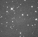
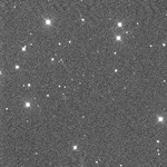
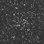
- The Field Star Removal page contains six panels and we’ll start with the top three. The graph on the top-left shows the distribution of proper motions in Right Ascension for all stars, with the greatest concentration corresponding to the cluster stars. The top-right shows a similar distribution for proper motion in Declination. And the centre graph is a two-dimensional scatter plot of the proper motion distribution where you should see the majority of stars clumped together. Start by using the sliders above the two proper motion distribution plots to zoom in on the main cluster in the proper motion distribution. As you zoom in you will see a tight clump of stars revealed in the 2D scatter plot. Continue zooming until you can clearly see the edge of this tight central distribution. At this point, your top three panels should look similar to the figure below.
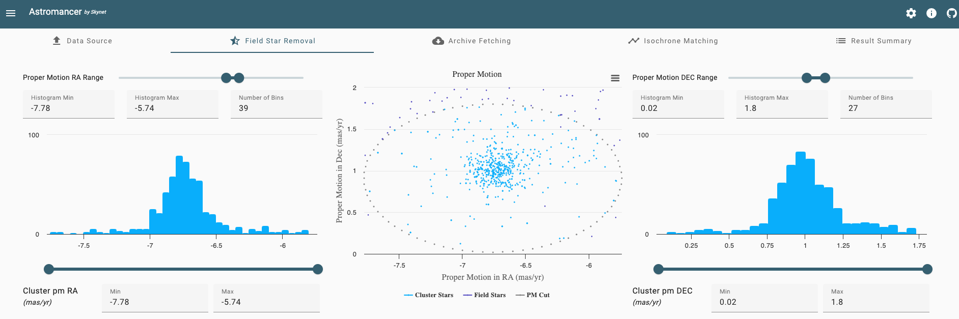
Figure 1: distribution of proper motions in NGC 3766 zoomed in on the cluster’s proper motion. - Next, use the sliders below the proper motion distribution graphs to adjust the Cluster pm RA and Cluster pm DEC ranges. This will affect the size of the ellipse in the 2D proper motion scatter plot, removing stars that are outside the ellipse as “field stars”. You are eventually going to add in a larger data set, incorporating all stars from Gaia that fall within your proper motion cut, so at this point you should be very liberal with the size of your ellipse. Make sure it’s set well outside the apparent proper motion bounds of the cluster (e.g. you might set the range in pm RA to -7.3 to -6.2 mas/yr and the range in pm DEC to 0.3 to 1.7 mas/yr).
- Scroll down to the bottom of the Field Star Removal page so you can apply similar cuts in distance. This all happens with the center Cluster Distance distribution plot. Again, start with the Distance range, bringing the top sliders in to roughly 1.5 to 3.0 kpc. Then bring in the Cluster Distance range sliders at the bottom to similarly liberal limits.
Note: on the far side of the peak in the distance distribution especially, it is advisable to be liberal when setting the limits. Gaia’s distance measurements have greater uncertainty at larger distances than for nearby stars with larger parallax, and we don’t want to exclude too many potential cluster stars with large distance uncertainty. 1.7 to 2.7 kpc seems to be a good range to use for this data set. - While there are still two steps in the full Clustermancer analysis, in the rest of this example we are going to leave those and instead explore two interesting pieces in our results up to this point: the proper motion and color-magnitude distributions.
- First, scroll up to view the Proper Motion scatter plot. Below the plot click “Cluster Stars” and “PM Cut” so the cluster stars and the proper motion boundary ellipse are removed from the graph. With these removed, if you set your cluster distance limits to reasonable values below you should see a continuous distribution of field stars here. To see what would happen if you were too conservative or too strict with your cluster distance limits, try the following:
- Scroll down to distance cuts and set the min distance to 2.2 kpc and the max distance to 2.7 kpc (you don’t need to use the sliders for this; you can just enter the numbers into the fields below). Now, when you look back at the proper motion scatter plot you should see a clump of cluster stars that have been removed from the data set.
- Scroll back down to the distance histogram and first set the Histogram Min to 0 and Histogram Max to 10 (in the fields above the graph). Then, below the graph set the Min value to 0 and the Max value to 10. Now, when you scroll up you should see a hole in the proper motion scatter plot, as we’ve added all the field stars, both between us and the cluster and on the far side of the cluster, to the group of “cluster stars”.
- The lesson in exploring these two extremes is that we can use the proper motion scatter plot not only to discover the cluster stars in proper motion space, but also to verify our cluster distance limits and ensure our constraints are too strict or too loose. This is because the distribution of proper motions in Milky Way field stars which are not at the cluster’s distance and comoving with the cluster (i.e. the cluster stars) should be continuous.
- You can now set the Cluster distance limits back to 1.7 and 2.7 kpc and re-enable Cluster Stars and the PM Cut on the scatter plot.
- The other graph to explore on this page is the color-magnitude diagram at the lower-left. At the top-right of the plot, click the three horizontal lines and “Download PNG image”. (Note: there should be a star of particular interest hiding behind the three lines at the top-right, so please download rather than screen shot the image). Now go back to Afterglow so you can make a color image and compare this to the cluster’s color-magnitude diagram:
- In Afterglow, select the B, V and R images.
- Above the list of images, click the three vertical dots and select “Group selected files” and confirm in the pop-up that you want to group these files.
- Right-click on each of the images and select the blue color map for the B image, green color map for V, and red color map for R.
- Click the top-level combined image, NGC3766.fits, and on the bottom-right click the “Zoom To Fit” button. You should now see a full color image of NGC 3766. This image is not yet a final product (we will get to that in Example 1.2 below). However, you should already be able to compare this image qualitatively with the color-magnitude diagram you produced in the previous step (which you should open now):
- In the tri-color cluster image, you should see two bright orange red giant stars. If both stars were selected as photometry sources (you would have had to manually select these as sources), they should show up as distinct points on your color-magnitude diagram, where the brightest sources are plotted at the top and the reddest sources are plotted on the right. On your color-magnitude diagram, you should therefore see these two stars plotted at the top-right. And since these two stars survived field star removal, you know that they are in fact cluster stars.
- It’s worth clarifying that we know the cool (i.e. red), luminous stars that are located towards the upper-right of the color-magnitude diagram are “giants” because the sizes of stars vary as
 . Therefore, the largest stars must be those with high luminosity and low temperature, and we call these stars “red giants”. We will discuss these giant stars further when we come to Examples 1.5 and 1.6 below.
 - On the top-left of the color-magnitude diagram, you should see a number of bright blue stars that gradually get redder as they get dimmer, just as you see in the image.
- Note that many of the stars in the image are not cluster members. In fact, if you return to Clustermancer and widen your cluster proper motion and distance constraints you will see several stars of all colors and magnitudes plotted on the color-magnitude diagram. The field stars are at varying distances, so do not follow the same color-magnitude trend as the cluster stars (e.g. nearby stars with low luminosity may be relatively bright compared to stars in the cluster with similar luminosity). The main takeaways here are that:
- the color-magnitude diagram is a quantitative graphical representation of the variability in color and magnitude that you see when looking at a color image of a star cluster, and
- star clusters exhibit trends in magnitude-color space that can be useful when attempting to isolate cluster stars from field stars, as these trends should become more apparent once the field stars have been removed; therefore,
- along with the proper motion scatter plot, the color-magnitude diagram should be used to aid in field star removal, by attempting to isolate the cluster stars that fall along the relatively tight correlations in color-magnitude space.
- Please leave both Clustermancer and Afterglow open with your image and field star removal limits set as you proceed to the next example.
In the next example, you will learn how to fit a physical model to that trend you identified above in NGC 3766’s HR diagram. This model, known as an isochrone model, plots the positions of stars that are all at a given distance, whose light is scattered by the same amount of interstellar dust, that are all the same age and have the same chemical composition, but which all formed with different masses. Therefore, isochrone models essentially show the positions of stars of different masses that are all part of the same cluster, so by adjusting parameters to fit the isochrone model to a cluster’s color-magnitude data, we can actually estimate the common physical properties of all stars in the cluster—i.e. their distance, age, chemical composition, and the amount of light from them that’s been obscured by dust.
In essence, we can learn a lot of information about a star cluster by plotting its stars’ positions on a color-magnitude diagram and fitting an isochrone model, all because we understand the physical causes of brightness and temperature differences among stars of different masses. And because science is super cool, and astronomy in particular is the coolest!
Example 1.2: NGC 3766 analysis, part b
In this next example, you are going to learn the steps to actually fit the isochrone model to the NGC 3766 cluster HR diagram you began creating in Example 1.1. If you have not yet worked through Example 1.1, please go back and follow the steps to create your graph, as these instructions will pick up from where we left off.
- To proceed, start by skipping past Archive Fetching and select “Isochrone Matching” from the stepper menu in Clustermancer.
- At the bottom-left, in the filter selection area, select the Blue filter to be B, the Red filter to be V, and the Lum filter to be V, then click Add, and at the bottom ensure “CM” is selected in the CM/HR toggle. You should now see a color-magnitude diagram (specifically, V magnitude plotted vs B-V color index), with an isochrone curve on the graph that by default does not pass through the cluster stars.
- Before attempting to fit the isochrone model to the data, there are a few properties of color-magnitude diagrams and HR diagrams, a few model parameters that should be explained, and a few general terms that we should define, to ensure you understand how to properly fit these models:
- The two axes of the diagram are plotted in magnitude units, and you can toggle between displaying the data in a color-magnitude diagram or in an HR diagram.
- The apparent magnitude measured from the flux of starlight in each image is calculated as
(1.1)

where
 is the photometric filter (in this case, the filters used were
  and
and  ),
),  is the flux of light measured in the -filter (essentially, the number of photons observed from a particular star), and
  is the image zero-point, a reference flux for the filter determined by calibrating to a reference catalogue to determine the dimmest flux measurable in your image.
 - Since the stars in a cluster are all at the same distance, it is possible to calculate the stars’ absolute magnitudes (analogous to luminosity) using the distance-modulus equation,
(1.2)

where
 is the galactic dust extinction in the band.
 - If the amount of galactic dust extinction is known, it can be used to calculate the stars’ intrinsic colors
 from their apparent colors
  which have been reddened by interstellar dust.
 - Thus, Clustermancer can take calibrated apparent magnitudes
 from your afterglow photometry file and use the distance
  and galactic dust extinction
  parameters you set with the sliders on the left-hand panel, and calculate each star’s absolute magnitude
  and intrinsic color .
 - Whereas a plot of magnitude vs apparent color is called a color-magnitude diagram, a plot of absolute magnitude/luminosity vs intrinsic color/surface temperature is an HR diagram. You can toggle your graph between the color-magnitude diagram and the HR diagram using the CM/HR toggle at the bottom-left.
- The apparent magnitude measured from the flux of starlight in each image is calculated as
- The horizontal axis plots color as photometric color index, which is defined as the difference in magnitude values measured for the same star using different filters; e.g. you should currently have plotted the
 color index. Since the magnitude scale is inverted (so lower magnitude values correspond to brighter fluxes; see the sign in Equation (1.1)), this means will be negative if a star is brighter when observed through the filter (which transmits blue light) than when observed through the filter (which transmits green light). Conversely, the star will have a positive color index if the star is brighter in than it is in .
 - Since stars emit thermal radiation with nearly blackbody spectra, color is analogous to temperature; e.g. with blue stars being the hottest ones, which emit more light at the blue end of the spectrum than the red.
- Most stars in NGC 3766 fall along the main sequence, the line connecting the hottest, most luminous (bright blue) stars at the top-left to the coolest, least luminous (dim red) stars at the bottom-right. These stars are all fusing hydrogen in their cores, and they mainly differ from one another by mass, with the most massive stars at the top-left and least massive at the bottom-right.
- The main sequence is not a thin line, as you might expect since all the stars are the same age, they have the same chemical abundance and they are located at the same distance. In fact, the differences in these quantities are so small that they are actually negligible. You might then think that the scatter is due to data quality, but the magnitude measurements in your data set, particularly of the brightest stars, are far more accurate than the amount of scatter you see. The source of scatter in your main sequence actually primarily comes from unresolved binary star systems.
- Typically, roughly half the stars in a cluster are members of binary star systems, and since the clusters are so far away, we don’t resolve the individual stars but see their combined light. For instance, if two stars have the same color and luminosity, they appear in the HR diagram with the same color but with brighter magnitude. If one star is lower mass than the other, the combined light of the two will be redder and brighter than that of the more massive star. As a result, the points in your HR diagram representing unresolved binary star systems create roughly a magnitude of scatter above the curve of isolated main sequence stars. Therefore, when we fit isochrone models to cluster data we must fit the curve to the densest part in the bottom of the main sequence.
- The top-left stars are the most massive main sequence stars in the cluster. Massive stars consume their core hydrogen fuel more rapidly than less massive stars, and the stars at the very top of the main sequence have nearly exhausted their fuel supply. When they do, their luminosity increases while their surface temperature cools and they become red giants, moving to the upper-right of the HR Diagram.
- In Clustermancer, select the HR toggle, then Standard View (top-right). Then, move the log(Age (yrs)) slider to larger values while holding the other parameters constant. You should see that the curve describing the main sequence remains roughly constant, while the point where stars leave the main sequence and migrate to the upper-right makes its way down the main sequence with increasing age. Therefore, this turn-off point at the top-left of the main sequence is what we use to determine a cluster’s age.[4]
- Astronomers are funny. We call all elements heavier than hydrogen and helium “metals”, and therefore denote our measure of the abundance of all elements heavier than hydrogen and helium as a star’s metallicity.
- In Clustermancer, select the HR toggle then move the metallicity slider to larger values while holding the other parameters constant. You should see that by increasing the metallicity, the isochrone model’s main sequence burns brighter and cooler (redder), and the giant branch becomes more evolved as the more “metal rich” clusters burn with higher luminosities to compensate for the extra shielding the metals add to core fusion reactions.
- When light travels from a cluster towards Earth, it must pass through interstellar dust. This galactic dust scatters some of the light so it never reaches us, and in fact preferentially scatters blue light, so clusters eventually appear both dimmer and redder when viewed from Earth. The parameter that measures interstellar reddening is denoted E(B-V) and is measured in magnitudes. Interstellar reddening is typically proportional to the amount of interstellar extinction that occurs in a given band . For example, in the Milky Way, we find on average that
 , whereas the proportionality constant
  is higher when relating reddening to extinction in bluer wavelength bands and lower for redder bands. Therefore, we require only one parameter, i.e. E(B-V), to describe both interstellar extinction and reddening.
- In Clustermancer, select the HR toggle then move the E(B-V) slider to larger values while holding the other parameters constant. As you increase E(B-V) in the plotting tool, notice that the data points on your graph become both brighter (they move up) and bluer (they move left). Thus, the graphs plot extinction/reddening-corrected values of absolute magnitude and color.
- All of these physical parameters—the distance, age, metallicity, reddening, and extinction—affect the form/location of the isochrone model within the color-magnitude diagram/HR diagram. And unfortunately they are all somewhat degenerate with one another—a change in one parameter can mimic a possible change in another. By observing the cluster in more than one filter, we can eliminate some of this degeneracy by plotting multiple data sets and fitting the isochrone simultaneously to them all.
- In Clustermancer, create a second plot of
 -band magnitude against
  color index by setting “Blue” as
  , setting “Red” as , and setting “Luminosity” as , then clicking Add.
 - Note that Clustermancer supports creating up to four color-magnitude diagrams/HR diagrams at once, and the placement can be adjusted by moving the corresponding boxes up or down at the bottom-left, or graphs can be removed by clicking the X.
- In Clustermancer, create a second plot of
- In the demonstration video below, we quickly review all the key points in this list before moving to the next step where you will see how to determine the physical parameters of NGC 3766 by matching the isochrone model to your stars in Clustermancer. Then, we will return to Afterglow Access to finalize our tri-color image using tools that set color balances based on the calibrated magnitudes of stars in each filter and even remove the effect of reddening to create a natural color image that shows us what the cluster would look like from Earth if there weren’t any dust along our line of sight.
- The two axes of the diagram are plotted in magnitude units, and you can toggle between displaying the data in a color-magnitude diagram or in an HR diagram.
- Match the isochrone model to your photometry data in Clustermancer:
- Note that below the distance slider you should see the cluster distance that is indicated by Field Star Removal (FSR). If you step back to the Field Star Removal page, you should see that this distance corresponds with the peak in the distance distribution. Move the slider to this value.
- At this point, if you have HR diagrams displayed it is recommended to select the Frame on Data option.
- Increase both age and metallicity to find a shape that is close to the shape of the data set you see. Metallicity should be somewhere approximately close to 0 for open clusters. Then adjust E(B-V) to bring the cluster data closer to your isochrone (HR diagram) or to bring the isochrone closer to the cluster data (color-magnitude diagram). Then modify all three to create a good match, bringing the isochrone up to the bottom of the main sequence by adjusting metallicity, fitting the turnoff by adjusting age, and getting the properly shaped isochrone main sequence to coincide with the data by adjusting the reddening value.
- When you’ve found a good fit, save your V vs B-V color-magnitude diagram as a PNG by clicking the three horizontal lines at the top-right of the graph..
- Use the following tri-color image processing sequence in Afterglow Access:
- (from Example 1.1, open NGC 3766 BVRI images, group BVR, set color maps for the three layers)
- select the top layer of your grouped image “NGC3766.fits”
- select Afterglow’s Display tool
- click Color Composite Tools > Link All Layers (Pixel Value)
- click Color Composite Tools > Photometric Calibration, then in the Photometric Calibration window click “Measure zero points with field calibration”. When zero point calibration completes, click Calibrate Colors.
- Set Stretch Mode to Midtone, and click the Default Preset. Raise the Background Level Percentile to a value lower than the peak to darken the background. 15 is a good number for these sample images.
- Click Export Image as JPG to save this image. This is the photometric color calibrated image of NGC 3766, which displays realistic colors for the stars in this cluster as they appear from Earth.
- Now click Color Composite Tools > Photometric Calibration one more time, and then set the Extinction E(B-V) value to the value you determined in Clustermancer. Click Calibrate Colors, and you will see your graph update colors in the photometric color calibrated image, removing the effect of reddening so the image now displays the cluster as it would appear from Earth if all the intergalactic dust along our line of sight were removed.
- Click Export Image as JPG to save a copy of this image.
So far, we’ve passed over two steps in the Clustermancer analysis: Archive Fetching and Results Summary. Example 1.3 will help you complete your analysis of NGC 3766 by adding in these steps.
Example 1.3: NGC 3766 analysis, part c
- Open Clustermancer. Your browser should still have all your data, field star removal and isochrone parameters loaded, just as you left them in Example 1.2 above. If not, please work through Examples 1.1-1.2 so you have everything as you left it at the end of Example 1.2, step 4.
- Click on Archive Fetching. You are now going to load photometric data from some all-sky catalogues.
- Click the Add Catalog Stars button.
- If you’ve done a good enough job setting your field star removal constraints, so you have reasonably narrow ranges in proper motion and distance, you should be able to fetch using the maximum radius, which is the default.
- In the Catalogues drop-down, select GAIA, 2MASS and WISE. Do NOT select APASS, as APASS contains some of the filters in your data set and the data will be combined with your data.
- Click Test Radius, and if there are fewer than the maximum number of stars the program will allow, you should see Fetch Data appear as an option. If so, click Fetch Data. If not, you will have to go back to the Field Star Removal step and tighten your proper motion and distance constraints, then come back and try the maximum radius again.
- Once Catalog Fetching is complete, you will see a new set of columns appear showing the number of cluster stars and field stars within the set radius in each of the catalogues you’ve fetched from.
- Go back to Field Star Removal and refine your proper motion and distance constraints. When you are happy with your constrains (refer to Example 1.1 for a refresher), move on to the Isochrone Matching page.
- On the Isochrone Matching page, close any graphs you have open and create an HR diagram with BP set as “Blue”, RP set as “Red” and RP set as “Lum”. Set the Max Error value to 0.05, and select Frame on Data.
- Refine your isochrone parameters, ensuring to fit model to the denser data at the bottom of the main sequence, ignoring the unresolved binary stars.
- Do not focus on any particular stars (e.g. the two red giants) to the detriment of your overall main sequence fit. Remember: you are working with real data and imperfect models here, and there are many factors that can lead to imperfection in your fit. The goal is to find a set of parameters that fits the data set overall as well as possible.
- When you are satisfied with your model fit, save the graph as a PNG and move on to the Result Summary page. Here, you will see several derived values listed based on your analysis: number of stars, physical radius (which comes from the angular size of the cluster and its distance), mass (which is calculated from the proper motion dispersion and radius of the cluster, i.e. based on the orbits of the stars within the cluster), among other parameters. Several graphs are also displayed, including an image showing the cluster’s location within a representative barred spiral galaxy that looks something like our Milky Way might look from a distance. Click the CSV button at the bottom-left and save a copy of the parameter values you just derived through your analysis.
In the Example 1.2, we noted that it is typically safe to assume that the stars in clusters are all at the same distance, they have the same metallicity, same extinction/reddening and they’re all the same age. But when do these assumptions not hold? And what impact do they have on our measurements when they do? These are questions we should address before moving on to have you image your own cluster and do your own isochrone modelling.
- Distance: if the cluster is so close to us that the distances between stars is a significant fraction of the distance to the cluster, we can expect more scatter in the cluster’s main sequence than we’d see from the multiple star systems alone. However, the sizes of clusters are typically only a few parsecs (for reference, note that the Orion nebula is only about 7 pc across), so even a nearby cluster a few hundred parsecs away will have negligible scatter due to distance.
- Age: Similar to distance, if the period of star formation within a cluster is a significant fraction of the cluster’s average age, then we should expect to see scatter. Star formation can last a few tens of millions of years, so if a cluster’s age is less than 100 million years (i.e. log(Age (yr)<8), the formation period may yet be up to 10% of the cluster’s total age. In this case, it is still important to fit the isochrone to the bottom of the main sequence, but we can expect more scatter above the curve than normal due to the presence of cool, luminous protostars.
- Metallicity: the molecular clouds that form star clusters are typically well mixed, so metallicity can typically be considered constant throughout a cluster. It is worth noting that in particularly large clusters (e.g. some of the more massive globular clusters, with ~106 stars), astronomers have found evidence of multiple star formation epochs. In this case, not only is there a broader range in ages, but due to the rapid life cycles of high mass stars we even see multiple populations with different metallicity. Such observations require spectroscopic analysis which is beyond the scope of this project, but it is worth noting that in such extreme cases the cluster’s ranges in both age and metallicity produce scatter about the average values you would expect to model with your own observations.
- Reddening/extinction: Interstellar reddening and extinction do often vary across a cluster, especially in active star forming regions where enough gas remains in the nebula to continue forming stars. The inhomogeneity of dust within our galaxy is typically enough to produce some scatter in a star cluster’s HR diagram, but the average value for a star cluster typically provides a good representation.
To summarize: we expect very little scatter in our data due to variability in distance and metallicity within a cluster, and we can expect somewhat more scatter due to variability in age and reddening/extinction. To give you a feel for how much scatter you could expect to see, in the next example you will apply the things you learned in Examples 1.1-1.3 to analyse a young open cluster where you can clearly see evidence of ongoing star formation.
Example 1.4: A Young Open Cluster, IC 2948
- Open Afterglow Access in a separate window and close any open images. You may discard changes. Open the four stacked BVRI images of IC 2948 located in the “Sample > MWU > Module 5 – HR diagrams > IC2948” directory.
- Create a tri-color image of this cluster, as follows:
- Click the Display tool on the right to move out of the Photometry tool.
- Select the B, R and V images from the file list and group them.
- Set your color maps for each image appropriately by right-clicking the image filename (B is blue, V is green, R is red). Zoom to fit.
- Under Color Composite Tools on the right, select Link All Layers (Pixel Value). Then, again under Color Composite Tools, select Photometric Color Calibration, then Measure zero points with field calibration. Leave all the default parameters and click Calibrate Colors once processing is complete.
- Change Stretch Mode to Midtone, then click the Faint Target button. You may adjust your background, midtone and saturation levels to remove any graininess in the image (e.g. in Percentile Mode, try background 6 and midtone 90), but in any case this provides a good sense of what you should expect in terms of age/star formation—i.e. the bok globules and cone nebula indicate there is still ongoing star formation in this region, the emission nebula clearly indicates you should expect some variable extinction/reddening.
- When you are happy with your color image, at the bottom-right click Export Image as JPG to save a copy of the image with colors calibrated using apparent magnitudes.
- Now, open the Clustermancer site. Rather than photometering the images in Afterglow and uploading those data, this time you are going to instead go directly to the catalog data. Under “Look Up a Cluster”, enter “IC 2948” and click the magnifying glass to search up the cluster’s coordinates.
- Click Test Radius to test the default radius value. You should see an error message stating that there are too many stars within the cluster’s radius. Reduce the search radius to 0.12 degrees and test again, then click Next to load the stars within this radius, then Next again to move on to Field Star Removal.
- IC 2948 is located in the Milky Way, so its proper motion is not as well isolated from the rest of the Milky Way field stars as the stars in NGC 3766. However, if you zoom the proper motion ranges towards the centre you should see a denser cluster of stars emerge in proper motion space, at around pmRA = -6 and pmDE = 0.65.
- Once you’ve located the denser patch of stars corresponding to IC 2948, adjust the limits of your PM cut, shrinking the ellipse around the cluster stars.
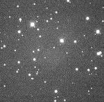
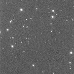
- Then scroll down and adjust your Distance Range first (in this case, 0-5 kpc works well), and then adjust the Cluster Distance sliders to better isolate the cluster’s main sequence and remove field stars. You may find it helpful to scroll up occasionally and disable Cluster Stars and PM Cut from the proper motion scatter plot, checking that the field stars have fairly uniform proper motion distribution. Eventually, your color-magnitude diagram should look similar to the one in Figure 2.
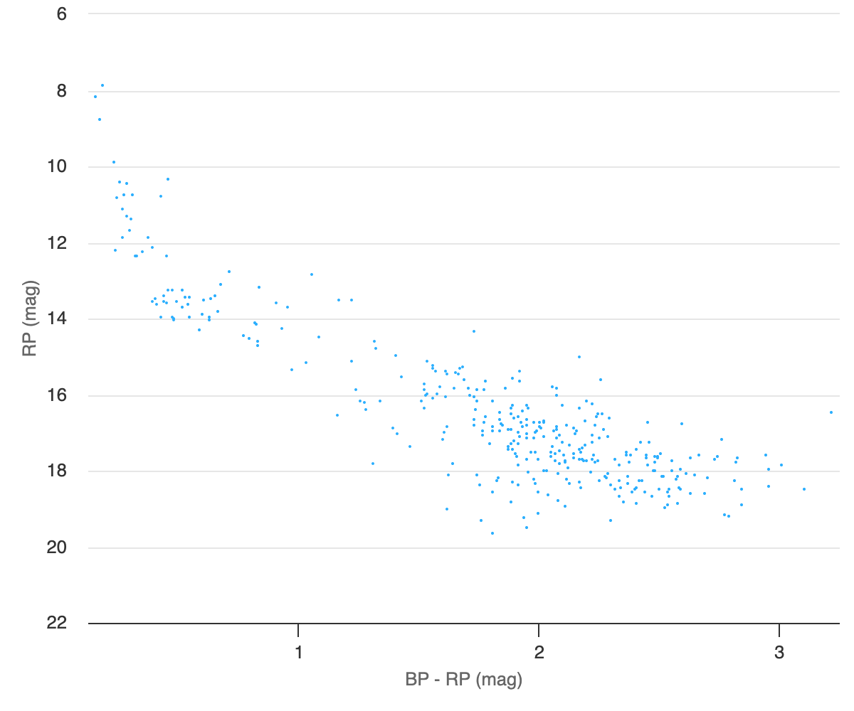
Figure 2: IC 2948 color-magnitude diagram. - Move to Archive Fetching and click Add Catalog Stars. Leave the default radius set to double the catalogued cluster radius, select the Gaia catalog, and then Test Radius.
- If more than 5000 stars fall within your proper motion and distance bounds, return to Field Star Removal and tighten your proper motion and distance constraints.
- If the radius test is successful, click Fetch Data to proceed.
- Return to Field Star Removal and adjust parameters until you are satisfied, then move on to Isochrone Matching. Now, do as follows:
- Create an HR diagram with RP vs BP-RP, and Frame on Data.
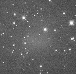
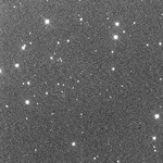
- Set Distance to 2.2 kpc, log(Age (yrs)) to 6.75, Metallicity to 0, E(B-V) to 0.34, and Max Error to 0.06. The resulting graph should look similar to Figure 3.
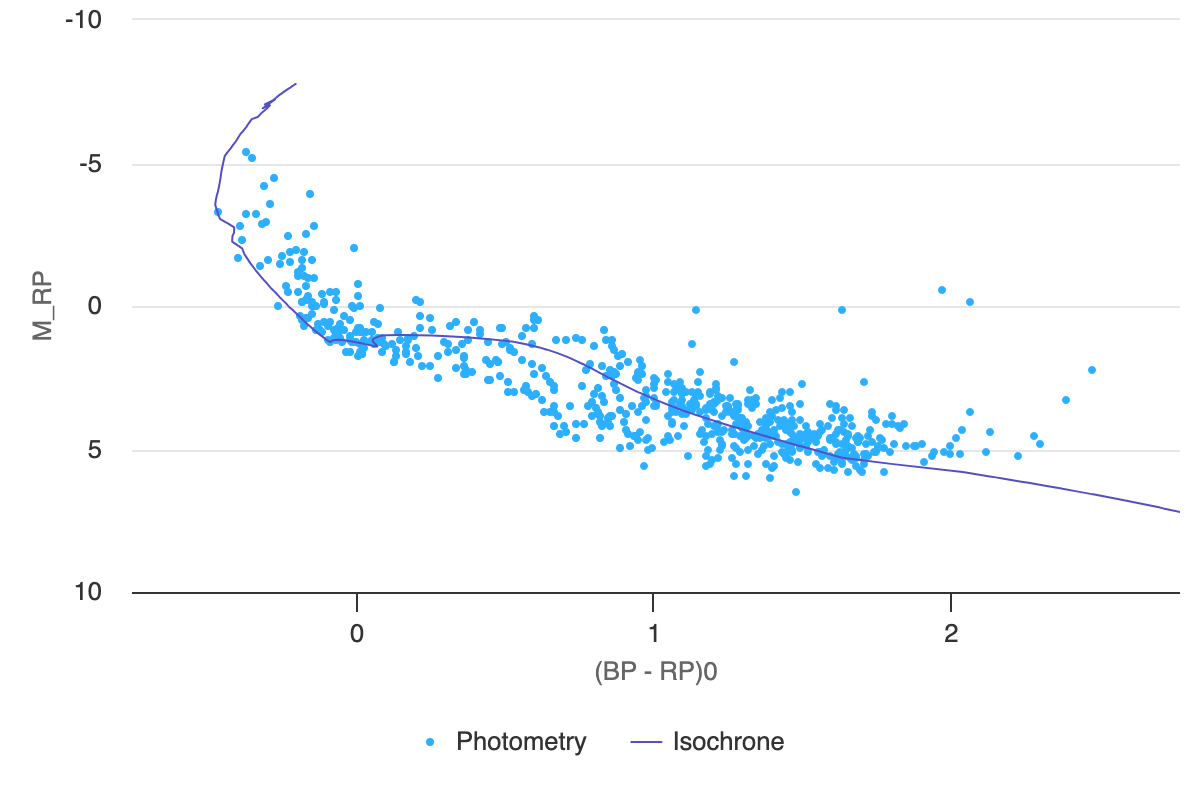
Figure 3: Gaia HR diagram of IC 2948. - Now, decrease log(Age (yrs)) to 6.6, using the down arrow. You should see the isochrone model move up to intersect younger pre-main sequence stars.
- Now, increase log(Age (yrs)) to roughly 8 to identify the oldest stars in this region, which have already settled onto the main sequence. As you do, also keep an eye on the most luminous stars as well, observing that the turnoff point in the isochrone model moves down and crosses through many of these blue giants as the model age increases.
- While the majority of stars in this cluster are still quite young, with ages of approximately 5 million years, this suggests that there has been continuous star formation in the region over ~100 million years.
- Adjust parameters to estimate “best fit” values. When you are satisfied with your model fit, save the graph as a PNG, then move on to the Result Summary page. Click the CSV button at the bottom-left and save a copy of the parameter values you just derived through your analysis.
- Return to Afterglow Access. With the E(B-V) value you estimated, you can now deredden your image of IC 2948. Click Color Composite Tools > Photometric Calibration, and set E(B-V) to 0.34, then click Calibrate Colors. Again, at the bottom-right of the image click Export Image as JPG to save a copy of your dereddened color image.
Our examples so far have focused on clusters that are dominated by main sequence and pre-main sequence stars, and we’ve taken care in the instructions to state that these are “young” stars which are fusing hydrogen into helium in their cores. Before moving on to collect your own observations of star clusters and trying to analyse them, you also need to understand what happens when stars evolve off the main sequence, and how this affects the HR diagrams of older clusters.
We’ve already discussed the main sequence turn-off point, and you saw in the above examples that this is important for determining the age of a cluster since stars at the turn-off point are those which have just run out of hydrogen in their cores, so they begin to evolve into old age. In the case of NGC 3766, the data you worked with contained two red giant stars, and you fit an isochrone model with a red giant branch that passed through those points. But our Galaxy also contains star clusters that are far older than the ones you’ve seen so far, and in these older clusters the red giant populations become far more important.
The oldest and largest clusters in our Galaxy are known as globular clusters. They contain ~105-107 stars and formed within the first few billion years of the Milky Way’s existence. Their orbits are oriented randomly within the galactic halo rather than being located in the disk of the Milky Way where we see open clusters and ongoing star formation, so we can see even very distant globular clusters because they are less obscured by interstellar dust.
Apart from the lowest mass stars in a globular cluster, the stars above roughly the Sun’s mass have all evolved to become giants. The sizes, ages and distances to globular clusters all amount to a distinctly different general HR diagram structure than the ones you’ve seen so far of young open clusters, for a couple of reasons:
- When star clusters form, it turns out that low mass stars form more often than high mass stars. Therefore, young open clusters contain relatively few stars massive enough to have evolved past the main sequence stage.
- High mass stars not only evolve from the main sequence more quickly than lower mass stars, but also have relatively short post-main sequence lifetimes, after which they die in supernova explosions and are soon no longer visible.
Therefore, young clusters tend to have very few giant stars in their HR diagrams, as these stars both die quickly and are less common in stellar populations. Eventually, more moderately-aged open clusters develop larger red giant populations as their turn-off points migrate down the main sequence and their giant populations suffer slower deaths. Relatively few of these old open clusters exist because the stars in lower mass clusters tend to disperse after ~109 years.[5] On the other hand, globular clusters have enough mass that they’ve survived since the formation of the Milky Way, and contain the oldest populations of stars. In fact, when we look at globular clusters, they typically contain several thousand giant stars spanning wide ranges in magnitude, and it can actually be difficult to make out the main sequence stars because of the great distances to these clusters and the fact that only the dim, red low-mass main sequence stars remain.
Globular clusters therefore provide the best information about the range of giant stars that form from stars of moderate mass:
- the red giant branch (RGB) stars that have exhausted their core hydrogen and are left with non-fusing helium cores, which grow in size and luminosity while their surface temperatures cool (recall that for stars,
 );
); - the horizontal branch stars which are now fusing helium in their cores, which are less luminous and smaller than the brightest RGB stars, but are also much hotter so they stand out as moderately bright, blue stars;
- and the asymptotic giant branch (AGB) stars which have exhausted their core helium fusion supply and now have inert carbon/oxygen cores. The luminosities and sizes of these stars increase while their surface temperatures cool, much as they did when they first left the main sequence and became red giants, and from the horizontal branch they asymptotically approach the red giant branch (where lower-mass stars with inert helium cores are now located).[6]
In the following examples, you will analyse both a moderately old open cluster and a globular cluster, to understand how to identify these populations when studying older clusters, as well as how to fit isochrone models to them.
Example 1.5: A Moderately Old Open Cluster, NGC 2682 (M67)
- Open Clustermancer and use the Look Up a Cluster dialog to search for M67. Reduce the radius to 0.5 degrees, Test Radius, and click Next, then Next again to load the cluster into the Field Star Removal tool.
- Note that there are two populations of stars displayed in the proper motion scatter plot! The denser and more numerous population, centered at (pmRA, pmDE) ~ (-11, -3.5) mas/yr is M67, while the less dense population of field star proper motions is centered around (pmRA, pmDE) ~ (-1.5, -2.5) mas/yr. You can easily verify this by adjusting your Cluster proper motion limits and comparing with the color-magnitude diagram in the bottom-left: the stars at (pmRA, pmDE) ~ (-11, -3.5) mas/yr have a well-defined main sequence and red giant branch, whereas the other population is a cloud of stars indicating a wide range of distances. Can you think of a simple explanation for why the two populations would have such different average proper motions?
- Isolate the cluster’s proper motion and distance ranges as you’ve done in examples 1.1-1.4 above, leaving some extra space as you still need to fetch the rest of the archival data and can then refine limits. Don’t worry that there are some stars to the upper-left of the turnoff point in the color-magnitude diagram.
- Move to Archive Fetching, click Add Catalog Stars, and again select only the Gaia catalogue. Test Radius, and if it fails return to tighten up your proper motion and distance limits. If the catalogue data successfully load, return to refine field star removal. When you are satisfied, proceed to Isochrone Matching.
- Create the Gaia HR diagram: RP vs BP-RP. Ensure you have the Max Error value set to at least 0.15 so the three stars at the bottom-left are displayed. These are white dwarfs, the dead carbon/oxygen cores of low-mass stars that have exhausted their core hydrogen and helium fuel and previously shed off their outer layers as planetary nebulae. It is important to note that while these are in fact cluster members, you should not attempt to fit the isochrone model to these stars.
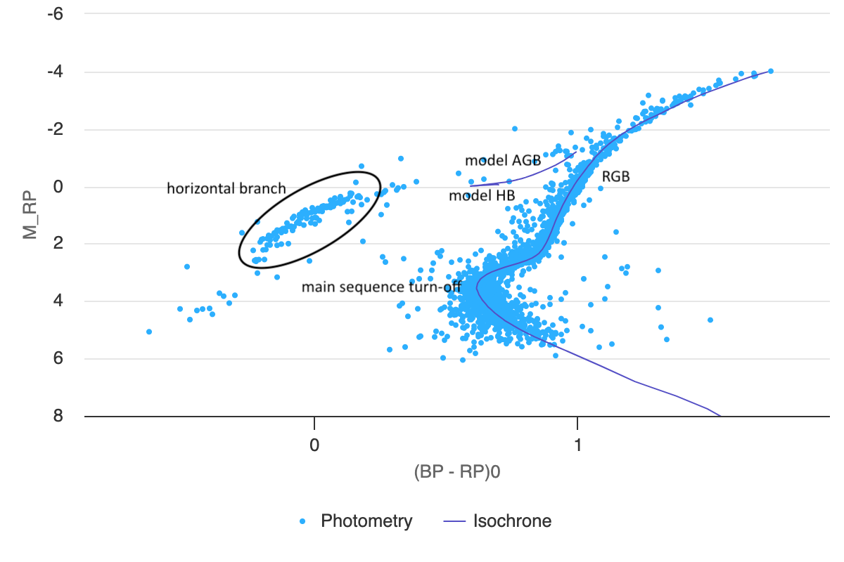
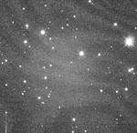
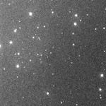
- Adjust distance (FSR mean is given, but you may also want to check the distribution on the FSR page), age, metallicity, and E(B-V) to find the set of parameters in which the isochrone model passes through the denser, single star main sequence population, up through the turnoff point and along the giant branch, and has a compact horizontal branch population at the bottom of the asymptotic giant branch. Your graph should look similar to the one in Figure 4 (though without the annotation). Download your own PNG image of this HR daigram.
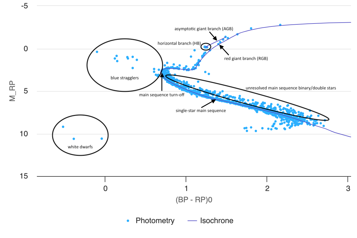
Figure 4: annotated Gaia HR diagram of M67. - Proceed to the Results Summary page where you will find estimates of the cluster’s number of stars, mass, radius, velocity dispersion, central location, as well as the parameters you entered, as well as tables of individual star data that you can download. Click Download Sources to download a csv containing astrometry and photometry data for all the stars in this cluster. Click the CSV button at the bottom-left and save a copy of the parameter values you just derived through your analysis.
- Now, open Afterglow Access in a separate window and close any open images in your Workbench. You may discard changes. Open the four BVRI images of NGC 2682 (M67) located in the “Sample > MWU > Module 5 – HR Diagrams > NGC2682” directory. With the E(B-V) value you estimated, you can now create a tri-color de-reddened image of this cluster:
- Group the BVR images and color each one appropriately, by right-clicking each image file.
- Click Color Composite Tools > Link All Layers (Pixel Value), then Color Composite Tools > Photometric Calibration, and click Measure zero points with field calibration.
- Enter the E(B-V) value you determined through isochrone matching, then click Calibrate Colors.
- Change the stretch mode to Midtone, click Default Preset, then tweak levels to your preference.
- At the bottom-right of the image click Export Image as JPG to download your dereddened color image.
- Comparing your color image to your Gaia HR diagram, you should clearly see the bright blue stars in the image that were plotted above the cluster’s turn-off point. In fact, with the data file you saved in step 6, you could identify these stars in your data set and locate them on the color image by cross-referencing their RA and Dec values. These stars are known as blue stragglers because they are massive blue stars that appear to have not evolved off the main sequence when the turn-off point reached them, so they are “straggling” behind. In general, it is important to ignore blue stragglers when fitting isochrone models because they are a result of evolutionary changes in binary star systems and are not accounted for by the models. However, their differences make them interesting stars to study![7]
- Note that so far, we’ve identified the unresolved binaries that lie above the single star main sequence, white dwarfs, and now blue stragglers as stars that should be avoided when matching isochrones to cluster HR diagrams.
NGC 2682 is a great example of a cluster with a well-defined main sequence, turn-off point and red giant population, and in many ways helps to bridge the gap between the young open clusters you analysed in Examples 1.1-1.4 and globular clusters like the one you will analyse in Example 1.6. In fact, this final example will both draw on the things you’ve learned about cluster HR diagrams and isochrone modelling throughout all the above examples and fill the last gaps in the knowledge you will need to be able to observe and analyse a separate cluster of your choosing.
While you will most likely find interesting peculiarities in any cluster you decide to observe, there are a few strategies you’ve learned so far to bear in mind as they will generally serve you well:
- Process is important: remove field stars first, as these “hide” the cluster within the color-magnitude diagram; and once the cluster’s proper motion and distance are better constrained, add archival data out beyond the cluster’s radius to ensure all cluster stars have are included in the data set and refine astrometric parameters (i.e. proper motion and distance); when matching isochrones, adjust the age and metallicity so that the isochrone model fits the shape of the turnoff point and red giant branch, and runs along the bottom of the main sequence; then adjust distance and reddening to align the model and data, ensuring the fit remains accurate when multiple photometric data sets are plotted; finally, refine parameters to get the best fit.
- Focus on the features near the top of the HR diagram, as these brighter stars should have more accurate measurements; and worry less about scatter towards the bottom of the HR diagram and fitting the model to those points since the corresponding measurements are less accurate.
- The isochrone model parameters may not be the same for all stars in a cluster, such as large globular clusters which are known to have formed stars in multiple epochs, resulting in multiple ages and metallicities, or young clusters in which different ages and extinctions are significant.
- Identify “special” stars like white dwarfs, unresolved binaries, and blue stragglers and ignore them as they are products of evolutionary paths that are not captured well by the isochrone models; in general, do not sacrifice a good fit to the majority of data points for the sake of a few stars.
- When using your own data, supplement yours with catalogued data. In most cases, Gaia photometry will be the most accurate data you can use, leading to the most accurate model parameter estimates. You should always strive for the most accurate results you can, using all data available to you.
All these points remain important when analysing globular cluster data. To them, we add the following which should also be taken into consideration in Example 1.6:
- In the case of a missing main sequence, or when the turnoff point is hidden within scattered data, focus on fitting the red giant branch (and, to a lesser extent, the asymptotic giant branch, though there will be relatively fewer stars in this shorter-lived evolutionary phase).
- A globular cluster’s horizontal branch will be far more prominent and spread out in its HR diagram than the tight clump of stars you found in the case of M67. At the same time, the horizontal branch is not well captured by our isochrone models, so you should avoid trying to force the model to fit these stars (e.g. see the HR diagram of the globular cluster M13 in Figure 5). The reason is that this relatively short phase of stellar evolution involves periods of instability and pulsation in which colors and magnitudes vary by up to a few magnitudes over periods of less than a day, so the horizontal branch is not easy to capture in a general evolutionary model. Instead, focus mainly on the red giant branch, fitting its average shape and that of the main-sequence turnoff (if present in the data).
- When removing field stars, do NOT try for a continuous distribution of field stars in your proper motion scatter plot. Gaia’s measurements for globular cluster stars have much higher errors than with open cluster stars, particularly when it comes to the lower luminosity stars and near the cluster’s core. Therefore, you will have to sacrifice a portion of probable cluster stars through relatively aggressive distance cuts in order to obtain an accurate sample for your HR diagram. Therefore, expect your scatter plot of “field star” proper motions to show a dense group where your “cluster stars” are located in this graph.
Example 1.6: A Globular Cluster, NGC 3201
Follow steps similar to those in Example 1.5 to analyse the Gaia catalogue data of NGC 3201 in Clustermancer, and analyse the sample images in Afterglow Access. Note that Afterglow photometry can be skipped entirely, as you did in the case of IC 2948 and M67. However, due to the density and number of stars in the cluster, you will likely need to go through multiple iterations of field star removal, archive fetching up to a limited radius, refinement of field star removal parameters, and subsequent archive fetching, before you can add all cluster stars out to the cluster’s full radius. Once you’ve isolated the stars in the cluster, complete your isochrone analysis using what you’ve learned above. When you have completed your analysis, enter the isochrone model parameters into this form.
Make sure to download your HR diagram(s) with isochrone fits, and save your Results Summary CSV when your analysis is complete.
Skynet Observations
Now that you have learned how to create a color image and analyse photometric data to determine a cluster’s age, metallicity, distance and reddening by fitting an isochrone model, you are going to close the loop by collecting and processing your own cluster observations. You will do this in two steps: you’ll start with cluster, telescope and filter selection, and then schedule an observation with the determined parameters; and then, once your images have come back, you will work through the basic image reduction steps needed to create stacked images which you can then photometer and combine into tri-colored images following the steps you learned in the Background section above.
Several factors are important to consider when selecting an astronomical target for observation, and before the target can actually be imaged. Regarding star clusters specifically, the cluster needs to be small enough that a large number of stars are visible within the telescope’s field of view; and yet, not so small, or so far away, that it can’t be effectively observed with the available equipment. It must also be observable with the telescopes you have available, at the time you plan to collect your images. For the purpose of your eventual analysis, you want to image the cluster through multiple filters across the visible spectrum. And you need to set your exposure lengths—which will be different for each filter—long enough that you collect good quality data for the cluster’s many dim stars while not overexposing the bright ones.
For this project to be manageable within the time that most classes have available for projects such as this, we have done our best to streamline the process as much as possible so you can work through and start collecting your data in just a few quick steps.
Where to observe
One of the most important and wonderful benefits of global telescope networks like the Skynet Robotic Telescope Network is that they enable us to observe from a range of latitudes, opening up the entire celestial sphere for potential observation. Another great benefit of robotic telescopes is that they self-monitor the weather and gather observations when conditions are right. Therefore, using telescopes from a global robotic network like Skynet means the only thing that keeps us from observing any target in the celestial sphere is the Sun. Typically, targets within a few hours of RA of the Sun are not observable (unless they happen to be circumpolar from a given telescope’s location). While stars closer to the poles tend to be observable even if the Sun is closer to the same RA, a good rule-of-thumb to use is that we should select targets that are at least 4 hours away from the Sun, and ideally more than 8 hours away.
Table 1.1 lists the Sun’s position on the first of each month, along with the maximum and minimum RA values that are typically observable on the same day, and the ideal range of RA values where you should aim to select your target for observation. Think about when you will be collecting your observations, whether you need them tonight, over the course of the next week, or in the coming month. Now, use Table 1.1 to interpolate the range in RA values where you should select your target.
Pro tip!
If observing with Skynet and it is critical that you collect your observations as soon as possible, choose a target whose RA is closer to the minimum value than the maximum value. Skynet’s observation queue will prioritize targets that are west of the meridian and on their way to setting in order to ensure that setting objects are observed and minimize airmass at the time of observation, so if your target is rising throughout the night your observation may sit a long time at the bottom of the queue.
Table 1.1
A list of the ranges in right-ascension at which objects are best observed during different months of the year. Generally, objects near the Min Target RA will set shortly after sunset on the given date, whereas objects near the Max Target RA will rise shortly before sunrise on that date. Targets within the Ideal RA Range are at least 8 hours of right-ascension from the Sun and will be observable over a longer period each night. Note that this table should be used as a guideline only, as a target's declination is also important. For example, targets at sufficiently high or low declination may be circumpolar, or even nearly circumpolar, and therefore observable year-round from some sites. In contrast, targets near the ecliptic must be furthest from the sun in RA in order to be observable.
| Date | Sun RA (hrs) |
Min Target RA (hrs) |
Max Target RA (hrs) |
Ideal RA Range (hrs - hrs) |
|---|---|---|---|---|
| 01-Jan | 18:50 | 22:50 | 14:50 | 2:50 - 10:50 |
| 01-Feb | 21:00 | 1:00 | 17:00 | 5:00 - 13:00 |
| 01-Mar | 22:50 | 2:50 | 18:50 | 6:50 - 14:50 |
| 01-Apr | 0:44 | 4:44 | 20:44 | 8:44 - 16:44 |
| 01-May | 2:35 | 6:35 | 22:35 | 10:35 - 18:35 |
| 01-Jun | 4:39 | 8:39 | 0:39 | 12:39 - 20:39 |
| 01-Jul | 6:43 | 10:43 | 2:43 | 14:43 - 22:43 |
| 01-Aug | 8:48 | 12:48 | 4:48 | 16:48 - 0:48 |
| 01-Sep | 10:44 | 14:44 | 6:44 | 18:44 - 2:44 |
| 01-Oct | 12:32 | 16:32 | 8:32 | 20:32 - 4:32 |
| 01-Nov | 14:28 | 18:28 | 10:28 | 22:28 - 6:28 |
| 01-Dec | 16:32 | 20:32 | 12:32 | 0:32 - 8:32 |
What to observe
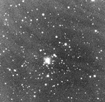
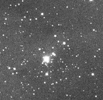
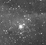
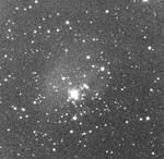
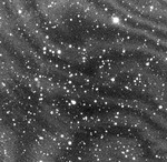
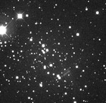
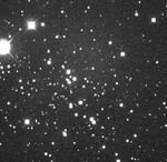
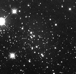
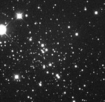
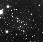
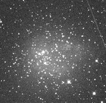
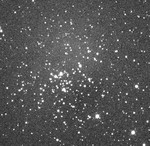
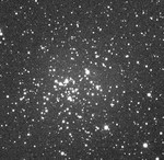
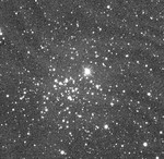
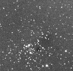
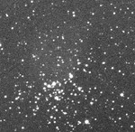
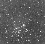
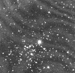
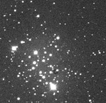
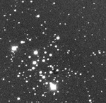
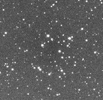
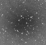
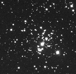
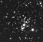
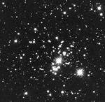
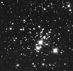
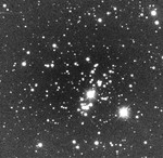
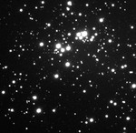
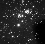
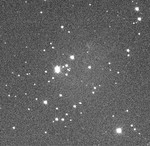
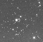
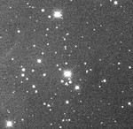
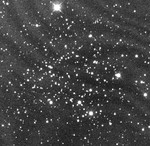
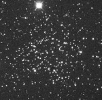
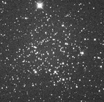
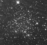
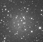
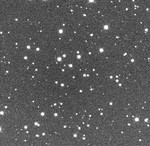
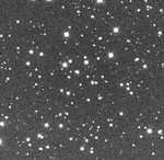
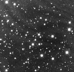
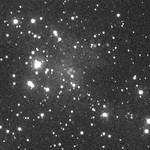
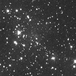
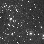
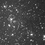
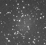
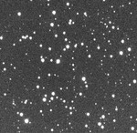
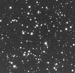
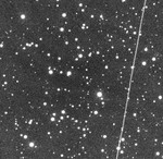
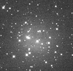
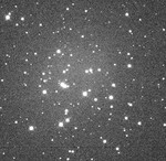
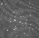
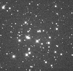
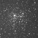
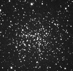
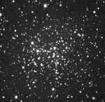
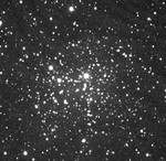
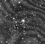
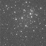
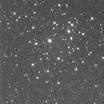
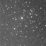
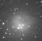
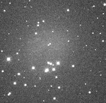
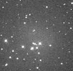
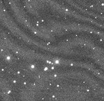
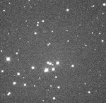
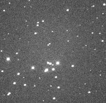
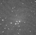
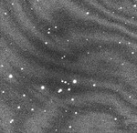
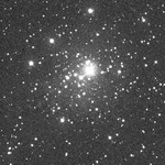
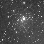
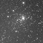
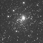
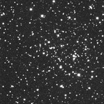
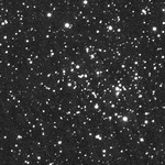
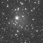
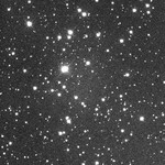
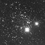
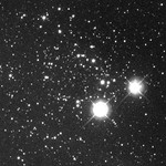
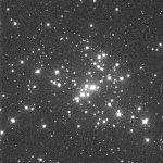
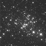
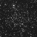
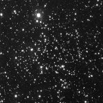
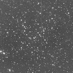
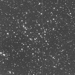
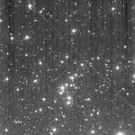
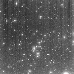
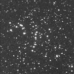
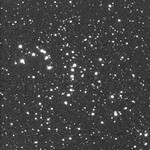
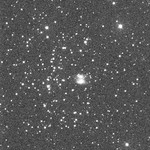
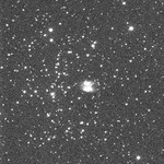
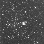
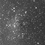
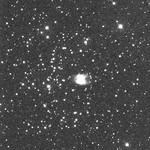
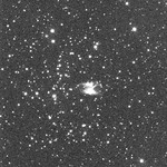
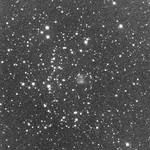
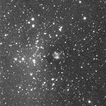
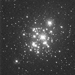
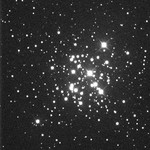
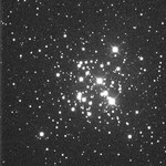
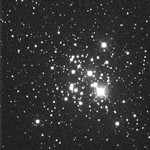
Once you have narrowed down a range of RA values for your target selection, navigate to the applicable rows of Table 1.2 if you will be observing an open cluster and/or the applicable rows of Table 1.3 if you will be observing a globular cluster. As you will see, these tables contain images of the clusters taken in multiple photometric bands, using Skynet’s PROMPT telescopes, with the exposure times displayed below each image. These exposure times have been optimized to enable you to collect quality photometric measurements through a wide range of magnitudes within the cluster, so we recommend submitting your observations with the listed exposure times. To improve data quality, when setting up your observation on Skynet we will recommend collecting at least 5 images per filter, which you can eventually combine to minimize error in your measurements.
When you have decided which cluster(s) you want to observe, move on to telescope and filter selection.
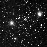
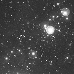
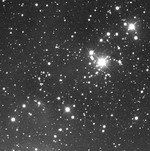
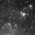
Table 1.2 Skynet Catalog of Small, Bright Open Star Clusters
A catalog of open star clusters, with coordinates, that have been imaged using Skynet PROMPT telescopes in various photometric filters. Images in this catalog represent what can be considered "good" images taken with the listed exposure times per filter, using Generic 16-inch telescope efficiency, and taken with a telescope with the field of view listed in the same row. To minimize noise in your color image and optimize photometric measurements, a minimum of 5 exposures per filter should be collected and stacked together.
**Note: Some clusters may be missing the sample images. That means that we are still testing them, and the suggested exposures may need to be adjusted. It's a fun challenge if you want to help us complete it!
***Note: The "Age" column is categorized where 'young' is log(Age)=8.
| Cluster Name | Age | RA (hr) |
Dec (deg) |
Telescope FoV | B | V | R | I | gprime | rprime | iprime | zprime |
|---|---|---|---|---|---|---|---|---|---|---|---|---|
| IC 1590 | young | 00:52:48.00 | 56:37:48.0 | 10'x10' |
 |
 |
 |
 |
 |
 |
 |
 |
| NGC 381 | intermediate | 01:08:25.92 | 61:34:44.4 | 10'x10' |
 |
 |
 |
 |
 |
 |
 |
 |
| NGC 457 | young | 01:19:37.20 | 58:16:48.0 | 10'x10' |
 |
 |
 |
 |
 |
 |
 |
|
| NGC 559 | intermediate | 01:29:31.20 | 63:18:07.2 | 10'x10' |
 |
 |
 |
 |
 |
 |
 |
 |
| NGC 581 | young | 01:33:15.84 | 60:39:07.2 | 10'x10' |
 |
30 s | 20 s | 8 s |
 |
20 s | 8 s | 15 s |
| NGC 637 | young | 01:43:06.48 | 64:02:42.0 | 10'x10' | 55 s | 25 s |
 |
15 s |
 |
15 s | 25 s | 40 s |
| NGC 654 | young | 01:43:58.80 | 61:54:00.0 | 10'x10' | 50 s | 25 s | 20 s | 22 s | 40 s | 20 s | 25 s | 45 s |
| NGC 663 | young | 01:46:12.00 | 61:13:30.0 | 10'x10' |
 |
 |
 |
 |
 |
 |
 |
 |
| NGC 744 | intermediate | 01:58:34.80 | 55:28:40.8 | 10'x10' |
 |
 |
 |
 |
 |
 |
 |
 |
| NGC 869 | young | 02:18:57.60 | 57:08:42.0 | 10'x10' |
 |
 |
 |
 |
 |
 |
 |
 |
| NGC 884 | young | 02:22:03.12 | 57:08:42.0 | 10'x10' | 40 s | 30 s | 20 s | 15 s |
 |
 |
25 s | 42 s |
| IC 1805 | young | 02:32:43.68 | 61:27:18.0 | 10'x10' |
 |
 |
 |
 |
 |
 |
 |
 |
| NGC 1039 | intermediate | 02:42:12.00 | 42:47:24.0 | 20'x20' | 13 s | 25 s | 10 s | 10 s | 7 s | 12 s | 10 s | 20 s |
| NGC 1027 | intermediate | 02:42:39.60 | 61:37:12.0 | 10'x10' |
 |
 |
 |
 |
 |
 |
 |
 |
| NGC 1245 | intermediate | 03:14:48.00 | 47:15:10.8 | 10'x10' |
 |
 |
 |
 |
 |
 |
 |
 |
| NGC 1342 | intermediate | 03:32:00.96 | 37:21:25.2 | 15'x15' |
 |
 |
 |
 |
 |
 |
 |
 |
| NGC 1528 | intermediate | 04:15:23.28 | 51:11:24.0 | 10'x10' |
 |
 |
 |
 |
 |
 |
 |
 |
| NGC 1647 | intermediate | 04:45:59.52 | 19:10:12.0 | 10'x10' |
 |
 |
 |
 |
 |
 |
 |
 |
| NGC 1664 | intermediate | 04:51:13.92 | 43:39:36.0 | 10'x10' |
 |
 |
 |
 |
 |
 |
 |
 |
| NGC 1817 | intermediate | 05:12:19.68 | 16:40:48.0 | 10'x10' |
 |
 |
 |
 |
 |
 |
 |
 |
| NGC 1893 | young | 05:22:49.68 | 33:25:48.0 | 10'x10' |
 |
 |
 |
 |
 |
 |
 |
 |
| NGC 1907 | intermediate | 05:28:04.80 | 35:19:30.0 | 10'x10' |
 |
 |
 |
 |
 |
 |
 |
 |
| NGC 1912 | intermediate | 05:28:51.60 | 35:48:00.0 | 10'x10' |
 |
 |
 |
 |
 |
 |
 |
 |
| NGC 1960 | young | 05:36:19.68 | 34:09:28.8 | 10'x10' |
 |
 |
 |
 |
 |
 |
 |
 |
| NGC 2099 | intermediate | 05:52:21.12 | 32:34:12.0 | 10'x10' |
 |
 |
 |
 |
 |
 |
 |
 |
| NGC 2112 | intermediate | 05:53:43.92 | 0:24:46.8 | 10'x10' |
 |
 |
 |
 |
 |
 |
 |
 |
| NGC 2129 | young | 06:01:06.24 | 23:20:24.0 | 10'x10' |
 |
 |
 |
 |
 |
 |
 |
 |
| NGC 2158 | intermediate | 06:07:25.68 | 24:05:31.2 | 10'x10' |
 |
 |
 |
 |
 |
 |
 |
 |
| NGC 2168 | intermediate | 06:09:12.48 | 24:21:36.0 | 10'x10' |
 |
 |
 |
 |
 |
 |
 |
 |
| NGC 2183 | young | 06:10:48.00 | -6:12:00.0 | 10'x10' |
 |
 |
 |
 |
 |
 |
 |
 |
| NGC 2194 | intermediate | 06:13:46.08 | 12:49:04.8 | 10'x10' |
 |
 |
 |
 |
 |
 |
 |
 |
| NGC 2215 | intermediate | 06:20:52.80 | -7:17:42.0 | 10'x10' |
 |
 |
 |
 |
 |
 |
 |
 |
| NGC 2244 | young | 06:31:55.20 | 4:56:24.0 | 20'x20' | 40 s | 35 s | 15 s | 15 s | 25 s | 15 s | 15 s | 30 s |
| NGC 2251 | intermediate | 06:34:37.20 | 8:22:12.0 | 10'x10' |
 |
 |
 |
 |
 |
 |
 |
 |
| NGC 2270 | intermediate | 06:43:58.80 | 3:28:12.0 | 10'x10' |
 |
 |
 |
 |
 |
 |
 |
 |
| NGC 2287 | intermediate | 06:46:03.12 | -20:44:42.0 | 20'x20' | 60 s | 40 s | 20 s | 20 s | 50 s | 20 s | 20 s | 40 s |
| NGC 2286 | intermediate | 06:47:39.12 | -3:09:18.0 | 10'x10' |
 |
 |
 |
 |
 |
 |
 |
 |
| NGC 2281 | intermediate | 06:48:18.00 | 41:04:48.0 | 10'x10' |
 |
 |
 |
 |
 |
 |
 |
 |
| NGC 2301 | intermediate | 06:51:46.80 | 0:27:54.0 | 10'x10' |
 |
 |
 |
 |
 |
 |
 |
 |
| NGC 2302 | intermediate | 06:51:52.32 | -7:04:48.0 | 10'x10' |
 |
 |
 |
 |
 |
 |
 |
 |
| NGC 2311 | intermediate | 06:57:46.80 | -4:36:36.0 | 10'x10' |
 |
 |
 |
 |
 |
|
|
 |
| NGC 2323 | intermediate | 07:02:43.20 | -8:22:12.0 | 10'x10' |
 |
 |
 |
 |
 |
 |
 |
 |
| NGC 2324 | intermediate | 07:04:10.32 | 1:02:16.8 | 10'x10' |
 |
 |
 |
 |
 |
 |
 |
 |
| NGC 2335 | intermediate | 07:06:50.40 | -10:01:48.0 | 10'x10' |
 |
 |
 |
 |
 |
 |
 |
 |
| NGC 2343 | intermediate | 07:08:04.08 | -10:36:00.0 | 10'x10' |
 |
 |
 |
 |
 |
 |
 |
 |
| NGC 2345 | young | 07:08:14.88 | -13:12:00.0 | 10'x10' |
 |
 |
 |
 |
 |
 |
 |
 |
| NGC 2354 | intermediate | 07:14:08.40 | -25:41:34.8 | 10'x10' |
 |
 |
 |
 |
 |
 |
 |
 |
| NGC 2355 | intermediate | 07:16:59.04 | 13:45:00.0 | 15'x15' |
 |
 |
 |
 |
 |
 |
 |
 |
| NGC 2360 | intermediate | 07:17:42.00 | -15:38:24.0 | 10'x10' |
 |
 |
 |
 |
 |
 |
 |
 |
| NGC 2374 | intermediate | 07:24:00.00 | -13:16:12.0 | 10'x10' |
 |
 |
 |
 |
 |
 |
 |
 |
| NGC 2414 | young | 07:33:08.88 | -15:27:18.0 | 10'x10' |
 |
 |
 |
 |
 |
 |
 |
 |
| NGC 2421 | young | 07:36:14.40 | -20:36:36.0 | 10'x10' |
 |
 |
 |
 |
 |
 |
 |
 |
| NGC 2422 | intermediate | 07:36:39.60 | -14:29:24.0 | 15'x15' | ||||||||
| NGC 2423 | intermediate | 07:37:06.72 | -13:51:00.0 | 10'x10' |
 |
 |
 |
 |
 |
 |
 |
 |
| NGC 2420 | intermediate | 07:38:23.04 | 21:34:01.2 | 15'x15' | 70 s | 35 s | 25 s | 25 s | 35 s | 20 s | 25 s | 50 s |
| NGC 2439 | young | 07:40:48.00 | -31:42:18.0 | 10'x10' |
 |
 |
 |
 |
 |
 |
 |
 |
| NGC 2437 215 | intermediate | 07:41:49.20 | -14:48:18.0 | 15'x15' | 50 s | 35 s | 20 s | 15 s | 25 s | 20 s | 20 s | 30 s |
| NGC 2447 | intermediate | 07:44:34.80 | -23:51:36.0 | 10'x10' |
 |
 |
 |
 |
 |
 |
 |
 |
| NGC 2477 | intermediate | 07:52:08.40 | -38:31:48.0 | 10'x10' |
 |
 |
 |
 |
 |
 |
 |
 |
| NGC 2479 | intermediate | 07:55:08.40 | -17:43:48.0 | 15'x15' |
 |
 |
 |
 |
60 s | 40 s | 40 s | 80 s |
| NGC 2482 | intermediate | 07:55:10.32 | -24:16:30.0 | 15'x15' |
 |
 |
 |
 |
30 s | 15 s | 30 s | 40 s |
| NGC 2489 | young | 07:56:18.72 | -30:03:57.6 | 10'x10' |
 |
 |
 |
 |
 |
 |
 |
 |
| NGC 2516 | intermediate | 07:57:57.60 | -60:45:00.0 | 15'x15' |
 |
 |
 |
 |
3 s | 2 s | 4 s | 8 s |
| NGC 2506 | intermediate | 08:00:00.00 | -10:45:36.0 | 10'x10' |
 |
 |
 |
 |
 |
 |
 |
 |
| NGC 2547 | young | 08:09:54.72 | -49:12:18.0 | 15'x15' |
 |
 |
 |
 |
3 s | 3 s | 5 s | 12 s |
| NGC 2539 | intermediate | 08:10:40.80 | -12:50:24.0 | 10'x10' |
 |
 |
 |
 |
 |
 |
 |
 |
| NGC 2548 | intermediate | 08:13:44.40 | -5:46:12.0 | 20'x20' | 50 s | 50 s | 40 s | 45 s |
 |
 |
 |
 |
| NGC 2567 | intermediate | 08:18:34.08 | -30:39:00.0 | 10'x10' |
 |
 |
 |
 |
 |
 |
 |
 |
| NGC 2571 | young | 08:18:56.64 | -29:44:06.0 | 10'x10' |
 |
 |
 |
 |
 |
 |
 |
 |
| NGC 2627 | intermediate | 08:37:19.20 | -29:56:42.0 | 10'x10' |
 |
 |
 |
 |
 |
 |
 |
 |
| NGC 2659 | young | 08:42:34.32 | -44:59:06.0 | 10'x10' |
 |
 |
 |
 |
 |
 |
 |
 |
| IC 2395 | young | 08:42:36.00 | -48:07:58.8 | 10'x10' |
 |
 |
 |
 |
 |
 |
 |
 |
| NGC 2669 | intermediate | 08:46:28.32 | -52:56:24.0 | 10'x10' |
 |
 |
 |
 |
 |
 |
 |
 |
| NGC 2682 | intermediate | 08:51:23.28 | 11:48:54.0 | 15'x15' |
 |
 |
 |
 |
30 s | 15 s | 15 s | 30 s |
| NGC 2818 | intermediate | 09:16:12.00 | -36:36:54.0 | 10'x10' |
 |
 |
 |
 |
 |
 |
 |
 |
| NGC 2910 | young | 09:30:28.80 | -52:55:30.0 | 10'x10' |
 |
 |
 |
 |
 |
 |
 |
 |
| NGC 2925 | young | 09:33:08.64 | -53:22:15.6 | 10'x10' |
 |
 |
 |
 |
 |
 |
 |
 |
| NGC 3114 | intermediate | 10:01:55.20 | -60:06:36.0 | 15'x15' |
 |
 |
 |
 |
7 s | 7 s | 6 s | 15 s |
| NGC 3293 | young | 10:35:49.20 | -58:13:48.0 | 10'x10' |
 |
 |
 |
 |
 |
 |
 |
 |
| NGC 3330 | intermediate | 10:38:45.60 | -54:06:54.0 | 10'x10' |
 |
 |
 |
 |
 |
 |
 |
 |
| NGC 3532 | intermediate | 11:05:49.20 | -58:43:48.0 | 20'x20' | 8 s | 8 s | 5 s | 10 s |
 |
 |
 |
 |
| IC 2714 | intermediate | 11:17:27.60 | -62:44:24.0 | 10'x10' |
 |
 |
 |
 |
 |
 |
 |
 |
| NGC 3680 | intermediate | 11:25:37.20 | -43:14:06.0 | 10'x10' |
 |
 |
 |
 |
 |
 |
 |
 |
| NGC 3766 | young | 11:36:18.00 | -61:36:54.0 | 10'x10' |
 |
 |
 |
 |
 |
 |
 |
 |
| IC 2948 | young | 11:39:12.72 | -63:30:36.0 | 15'x15' |
 |
 |
 |
 |
 |
 |
 |
 |
| NGC 3960 | intermediate | 11:50:38.40 | -55:40:12.0 | 10'x10' |
 |
 |
 |
 |
 |
 |
 |
 |
| NGC 4103 | young | 12:06:39.60 | -61:15:00.0 | 10'x10' |
 |
 |
 |
 |
 |
 |
 |
 |
| NGC 4349 | intermediate | 12:24:14.40 | -61:52:12.0 | 10'x10' |
 |
 |
 |
 |
 |
 |
 |
 |
| NGC 4609 | intermediate | 12:42:18.00 | -62:59:24.0 | 10'x10' | 40 s | 30 s | 20 s | 20 s | 20 s | 15 s | 20 s | 40 s |
| NGC 4755 | young | 12:53:38.40 | -60:22:30.0 | 10'x10' |
 |
 |
 |
 |
10 s | 10 s | 20 s | 40 s |
| NGC 4852 | intermediate | 13:00:10.80 | -59:35:24.0 | 10'x10' |
 |
 |
 |
 |
 |
 |
 |
 |
| NGC 5281 | young | 13:46:33.60 | -62:55:30.0 | 10'x10' |
 |
 |
 |
 |
 |
 |
 |
 |
| NGC 5316 | intermediate | 13:53:56.40 | -61:52:12.0 | 15'x15' |
 |
 |
 |
 |
 |
 |
 |
|
| NGC 5617 | intermediate | 14:29:47.28 | -60:42:54.0 | 15'x15' |
 |
 |
 |
 |
30 s | 15 s | 20 s | 40 s |
| NGC 5749 | intermediate | 14:48:46.80 | -54:29:06.0 | 10'x10' |
 |
 |
 |
 |
 |
 |
 |
 |
| NGC 5822 | intermediate | 15:04:28.32 | -54:23:24.0 | 20'x20' | 50 s | 30 s | 15 s | 15 s |
 |
 |
 |
 |
| NGC 5823 | intermediate | 15:05:31.20 | -55:35:42.0 | 10'x10' |
 |
 |
 |
 |
 |
 |
 |
 |
| NGC 5925 | intermediate | 15:27:34.32 | -54:31:01.2 | 15'x15' | 120 s | 60 s | 30 s | 30 s | 60 s | 30 s | 30 s | 60 s |
| NGC 6025 | intermediate | 16:03:16.08 | -60:24:00.0 | 15'x15' |
 |
 |
 |
 |
4 s | 4 s | 5 s | 20 s |
| NGC 6067 | young | 16:13:12.00 | -54:13:12.0 | 10'x10' |
 |
 |
 |
 |
 |
 |
 |
 |
| NGC 6124 | intermediate | 16:25:15.60 | -40:39:00.0 | 10'x10' |
 |
 |
 |
 |
 |
 |
 |
 |
| NGC 6134 | intermediate | 16:27:48.48 | -49:09:18.0 | 10'x10' |
 |
 |
 |
 |
 |
 |
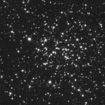 |
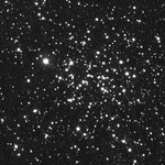 |
| NGC 6192 | intermediate | 16:40:21.12 | -43:21:36.0 | 10'x10' | ||||||||
| NGC 6231 | young | 16:54:14.40 | -41:49:48.0 | 10'x10' | ||||||||
| NGC 6242 | young | 16:55:33.60 | -39:27:36.0 | 10'x10' | ||||||||
| NGC 6253 | intermediate | 16:59:04.80 | -52:42:00.0 | 10'x10' | ||||||||
| NGC 6259 | intermediate | 17:00:54.00 | -44:41:24.0 | 10'x10' | ||||||||
| NGC 6268 | intermediate | 17:02:07.68 | -39:42:54.0 | 10'x10' | ||||||||
| NGC 6281 | intermediate | 17:04:40.80 | -37:58:48.0 | 10'x10' | ||||||||
| IC 4651 | intermediate | 17:24:54.00 | -49:56:06.0 | 10'x10' | ||||||||
| NGC 6494 | intermediate | 17:56:54.72 | -19:00:00.0 | 10'x10' | ||||||||
| NGC 6531 | young | 18:04:12.00 | -22:29:24.0 | 10'x10' | ||||||||
| NGC 6633 | intermediate | 18:27:20.64 | 06:30:00.0 | 20'x20' | ||||||||
| IC 4725 | young | 18:31:42.72 | -19:06:36.0 | 10'x10' | ||||||||
| NGC 6649 | intermediate | 18:33:21.60 | -10:24:00.0 | 10'x10' | ||||||||
| NGC 6705 | intermediate | 18:50:59.28 | -06:16:48.0 | 10'x10' | ||||||||
| NGC 6791 | intermediate | 10'x10' | ||||||||||
| NGC 6811 | intermediate | 19:37:22.08 | 46:23:42.0 | 10'x10' | ||||||||
| NGC 6819 | young | 19:41:16.80 | 40:11:42.0 | 10'x10' | ||||||||
| NGC 6823 | intermediate | 19:43:08.40 | 23:18:00.0 | 15'x15' | ||||||||
| NGC 6866 | intermediate | 20:03:56.88 | 44:09:36.0 | 10'x10' | ||||||||
| NGC 6939 | intermediate | 20:31:31.68 | 60:39:36.0 | 10'x10' |
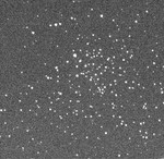 |
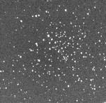 |
 |
 |
 |
 |
 |
 |
| NGC 6940 | intermediate | 20:34:26.40 | 28:16:48.0 | 10'x10' |
 |
 |
 |
 |
 |
 |
 |
 |
| NGC 7086 | young | 21:30:27.12 | 51:36:28.8 | 10'x10' | 100 s |
 |
 |
 |
25 s | 20 s |
 |
 |
| NGC 7128 | intermediate | 21:43:50.64 | 53:43:30.0 | 10'x10' |
 |
 |
 |
 |
 |
 |
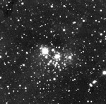 |
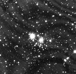 |
| NGC 7142 | intermediate | 21:45:12.72 | 65:47:31.2 | 10'x10' |
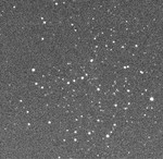 |
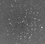 |
 |
 |
 |
 |
 |
 |
| NGC 7209 | young | 22:04:54.24 | 46:33:07.2 | 10'x10' |
 |
 |
 |
 |
 |
 |
 |
 |
| NGC 7243 | young | 22:15:10.80 | 49:52:30.0 | 10'x10' |
 |
 |
 |
 |
 |
 |
 |
 |
| NGC 7380 | young | 22:47:20.40 | 58:05:42.0 | 10'x10' |
 |
 |
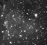 |
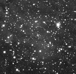 |
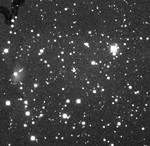 |
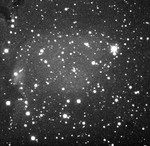 |
 |
 |
| NGC 7654 | intermediate | 23:24:42.48 | 61:38:13.2 | 10'x10' |
 |
 |
 |
 |
 |
 |
 |
 |
| NGC 7762 | intermediate | 23:49:51.60 | 68:01:30.0 | 10'x10' |
 |
 |
 |
 |
 |
 |
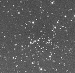 |
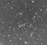 |
Table 1.3 Skynet Catalog of Bright Globular Clusters
A catalog of globular star clusters, with coordinates, that have been imaged using Skynet PROMPT telescopes in various photometric filters. Images in this catalog represent what can be considered "good" images taken with the listed exposure times per filter, using Generic 16-inch telescope efficiency, and taken with a telescope with the field of view listed in the same row. To minimize noise in your color image and optimize photometric measurements, a minimum of 5 exposures per filter should be taken and stacked together.
*Note: Times here are starting points based on the images shown. They may need to be adjusted.
**Note: Some clusters may be missing the sample images. That means that we are still testing them, and the suggested exposures may need to be adjusted. It's a fun challenge if you want to help us complete it!
| Cluster Name | RA (hr) |
Dec (deg) |
Telescope FoV | B | V | R | I | gprime | rprime | iprime | zprime |
|---|---|---|---|---|---|---|---|---|---|---|---|
| NGC 104 | 00:24:01.20 | -72:04:51.6 | 10' x 10' |
 |
 |
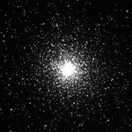 |
 |
 |
 |
 |
 |
| NGC 288 | 00:52:46.32 | -26:35:06.0 | 10' x 10' |
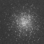 |
 |
 |
 |
 |
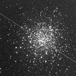 |
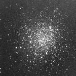 |
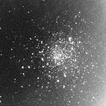 |
| NGC 362 | 01:03:18.00 | -70:50:49.2 | 10' x 10' |
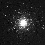 |
 |
 |
 |
 |
 |
 |
 |
| NGC 1261 | 03:12:16.32 | -55:12:57.6 | 10' x 10' |
 |
 |
 |
 |
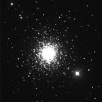 |
 |
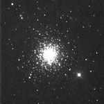 |
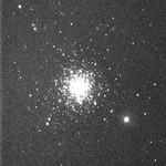 |
| NGC 1851 | 05:14:07.88 | -40:02:34.8 | 10' x 10' |
 |
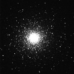 |
 |
 |
 |
 |
 |
 |
| NGC 1904 | 05:24:11.04 | -24:31:12.0 | 10' x 10' |
 |
 |
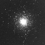 |
 |
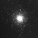 |
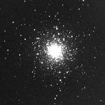 |
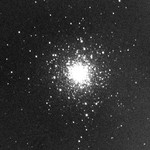 |
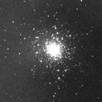 |
| NGC 2808 | 09:12:03.12 | -64:51:46.8 | 10' x 10' |
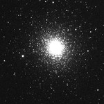 |
 |
 |
 |
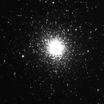 |
 |
 |
 |
| NGC 3201 | 10:17:36.96 | -46:24:43.2 | 10' x 10' |
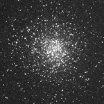 |
 |
 |
 |
 |
 |
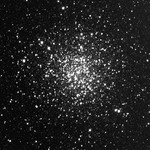 |
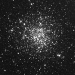 |
| NGC 4372 | 12:25:45.60 | -72:39:32.4 | 15' x 15' |
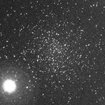 |
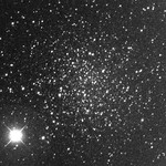 |
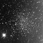 |
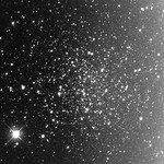 |
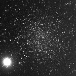 |
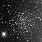 |
 |
 |
| NGC 4590 | 12:39:28.08 | -26:44:38.4 | 10' x 10' |
 |
 |
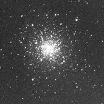 |
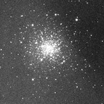 |
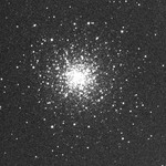 |
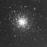 |
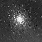 |
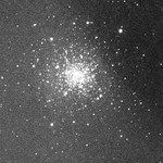 |
| NGC 4833 | 12:59:34.08 | -70:52:37.2 | 10' x 10' |
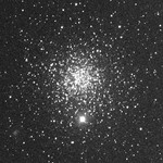 |
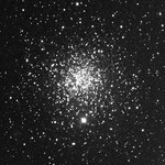 |
 |
 |
 |
 |
 |
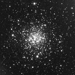 |
| NGC 5024 | 13:12:55.20 | 18:10:04.8 | 10' x 10' |
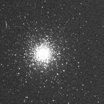 |
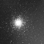 |
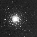 |
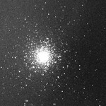 |
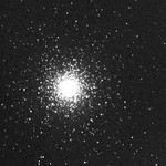 |
|
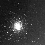 |
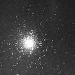 |
| NGC 5139 | 13:26:47.28 | -47:28:48.0 | 15' x 15' | ||||||||
| NGC 5272 | 13:42:11.52 | 28:22:37.2 | 10' x 10' | ||||||||
| NGC 5286 | 13:46:26.88 | -51:22:26.4 | 10' x 10' |
 |
 |
 |
 |
 |
 |
 |
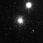 |
| NGC 5466 | 14:05:31.20 | 28:32:02.4 | 10' x 10' | ||||||||
| IC 4499 | 15:00:18.48 | -82:12:50.4 | 10' x 10' |
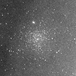 |
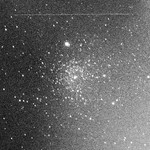 |
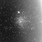 |
 |
 |
 |
 |
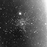 |
| NGC 5897 | 15:17:24.24 | -21:00:36.0 | 10' x 10' |
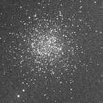 |
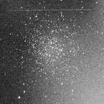 |
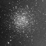 |
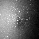 |
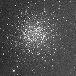 |
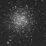 |
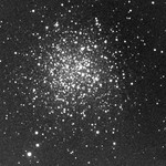 |
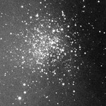 |
| NGC 5904 | 15:18:33.12 | 02:04:51.6 | 15' x 15' | ||||||||
| NGC 5927 | 15:28:00.96 | -50:40:22.8 | 10' x 10' |
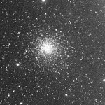 |
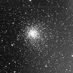 |
 |
 |
 |
 |
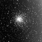 |
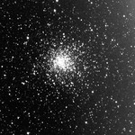 |
| NGC 6093 | 16:17:02.40 | -22:58:33.6 | 10' x 10' | ||||||||
Telescope and filter selection
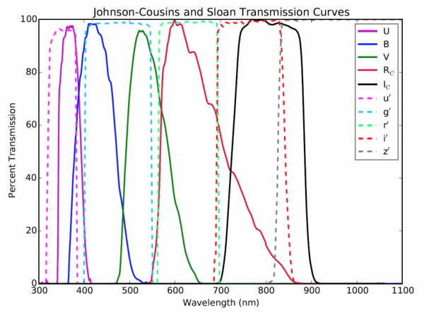
Before moving too far away from Tables 1.2 and 1.3, it is worth taking a moment to draw your attention to something you may have already noticed when scanning through the table. Namely, you should be able to see already in some sets of images which stars are particularly blue in color and which are particularly red in color. Since the B and gprime bands transmit blue light (see Figure 1), stars that are brightest in the B and gprime images will appear blue when combined with images from across the optical band. Similarly, stars that appear brightest in I, iprime and zprime, which therefore emit most of their light in the near-infrared, will appear red in a combined color image. In order to create combined color images, you will need to collect data in at least three bands that you can use as blue, green and red channels. However, adding an extra filter doubles the number of combinations you can use to create HR diagrams, from 3 to 6. And from the perspective of visualising the information in a color image, adding a fourth filter (e.g. adding I-band images to the groups created in Examples 1.1-1.6, with “heat map” used to colorize the image) often provides more useful information, particularly when studying young clusters.
For Skynet observations, it is recommended to use PROMPT telescopes only (unless your instructor advises otherwise). A list of currently available PROMPT telescopes on Skynet, the available photometry filters, and each telescope’s field of view are listed in Table 1.4.
Table 1.4 Skynet PROMPT Telescopes
| Telescope | Location | Field of View | Available Photometric Filters |
|---|---|---|---|
| PROMPT2 | Cerro Tololo Inter-American Observatory | 10'x10' | |
| PROMPT3 | Cerro Tololo Inter-American Observatory | 20'x20' | gprime, rprime, iprime, zprime |
| PROMPT5 | Cerro Tololo Inter-American Observatory | 10'x10' | B, V, R, I, gprime, rprime, iprime, zprime |
| PROMPT6 | Cerro Tololo Inter-American Observatory | 15'x15' | B, V, R, I |
| PROMPT-MO | Meckering Observatory | 10'x10' | B, V, R, I, gprime, rprime, iprime, zprime |
| PROMPT-USask | Sleaford Observatory | 10'x10' | B, V, R, I, gprime, rprime, iprime, zprime |
With the above in mind, and referring to the information in Tables 1.2 and 1.3 regarding recommended fields of view, available filters on the telescopes with the given field of view (i.e. where example images exist), and individual exposure lengths, you may now determine which telescope(s) and filters will be best to observe with.
Make a note of the name(s) of your target cluster(s), ALL telescopes you can use for your observations, the filters you will use (e.g. BVRI, BVr’i’, g’r’i’z’, etc), and the exposure times you will set for each filter. Once you have done that, move on to the next section where you will decide on your observing schedule and submit your observations!
Scheduling your observation
Before scheduling your observation, determine how many images you need to collect per filter. We recommend at least five, but ideally 10 or more if you have access to enough telescope time.
If observing with Skynet, you can calculate the number of credits your observation will require by multiplying the sum of exposure times in all filters by the number of observations in each filter. The number of Skynet credits your observation requires is equal to the total number of seconds of exposure time.
If you have more than a week to collect your data, follow the Image Sequence Method instructions below, which will return the best quality data. This method will enable you to collect data under a variety of conditions (focus, seeing, airmass, etc) and reject any bad images that come back, whereas the quicker dithering method described below should only be used if you are in a rush to collect data, as the images you collect may all be suboptimal.
Image sequence method
- Login to Skynet and navigate to My Observatory > Optical Observing > + Add New Observation. Type your cluster’s name in Target Lookup and click Search to bring up its coordinates.
- We recommend leaving max sun elevation and min target elevation at the default values of -18 and 30, respectively. Min visible hours won’t matter if you selected a target in the recommended RA range, so leave it at the default also.
- Set Max Moon Phase to 70 and Min Moon Separation to 60. Leave everything else as defaults.
- On the next two pages, select the filters you decided to observe with, and ALL available PROMPT telescopes with the field of view listed for your target in Table 1.2 or 1.3.
- On the next page, under Choose Exposure Efficiency, select Generic 16-inch.
- Set # Exps to 1 for each filter (regardless how many exposures you plan to collect, set this value to 1); set Duration(s) to the image duration values from Table 1.2 or 1.3 for your target.
- Under Advanced Options, select “All exposures on same telescope”
- Check “Repeat this observation…” and enter the number of times you wish to repeat the observation; i.e. the total number of exposures per filter you want taken. Typically, the amount of time between observations should be set to 1-2 hours to allow enough time for environmental conditions to change.
- Once you have set your number of repetitions and minimum delay duration, you will notice that the Credits Required for the observation has changed. Select a time account with sufficient credits or adjust the settings in step 9. When you are satisfied, click Save and Continue.
- Review your observation parameters on the final page, comparing them against the above steps, and click Submit when ready. Note that if you realize later that you did make a mistake, you can cancel the observation from your Observations List and recover any unused credits from the observation.
Dithering method
- Login to Skynet and navigate to My Observatory > Optical Observing > + Add New Observation. Type your cluster’s name in Target Lookup and click Search to bring up its coordinates.
- We recommend leaving max sun elevation and min target elevation at the default values of -18 and 30, respectively. Min visible hours won’t matter if you selected a target in the recommended RA range, so leave it at the default also.
- Set Max Moon Phase to 70 and Min Moon Separation to 60.
- Check Enable dithering with 3 x 3 grid and set arcsecond spacing to 10.
- On the next two pages, select the filters you decided to observe with, and ALL available PROMPT telescopes with the field of view listed for your target in Table 1.2 or 1.3.
- On the next page, under Choose Exposure Efficiency, select Generic 16-inch.
- Set # Exps to the number of exposures per filter you decided to collect for this observation; set Duration(s) to the image duration values from Table 1.2 or 1.3 for your target.
- Select a time account with at least the number of credits shown under Credits Required or adjust # Exps.
- Leave the default Advanced Settings. When you are satisfied, click Save and Continue.
- Review your observation parameters on the final page and click Submit when ready. Note that if you realize later that you did make a mistake, you can cancel the observation from your Observations List and recover any unused credits from the observation.
Advanced project
If you wish to observe a star cluster that is not listed in Tables 1.2 and 1.3, you may wish to explore the full Milky Way Star Clusters Catalog which is available in this Google Sheet. Catalogue data for the full list of clusters is not as good as what you’ve dealt with in the Note that many of the considerations discussed above will then apply; e.g. you should choose a cluster whose estimated size is comparable to your telescope’s field of view and ensure it is currently observable with your equipment. To get a better idea what the cluster will look like within your field of view, you should search for it at Aladin Lite and zoom to the appropriate field size. Once you have selected a target, rather than estimating optimal exposure times as in Tables 1.2 and 1.3, we recommend instead observing with 3 s, 30 s, and 300 s exposures in all the filters you plan to observe with. Each set of images taken with the same filter and exposure duration should then be aligned and stacked following the instructions in the next section. Once you have these stacked images prepared, extract sources from one of the 300 second exposures and click on the bright, saturated stars to ensure they are selected as well, as you’ve done in the examples in the background section. You’ll therefore have three images per filter you observed with, and should batch photometer all of them at once. When you have your batch photometry file, it will contain a lot of bad values where stars were saturated or not enough flux was present, and often there will be multiple measurements per filter for a given star. To clean up your afterglow_photometr.csv file, go to this Google Colaboratory workbook and login to your Google account. Save a copy to your drive where you can edit or run it. And then follow the instructions written at the top of the workbook to run the code and clean up your file before moving on to your Clustermancer analysis.
Image Processing
When your observation is complete, you can process your images to produce aligned, stacked images in each filter with reduced noise. In this section, you will learn the process of image stacking, which is the last piece needed before you can create combined color images and HR diagrams with your own data, following the procedures you learned in the Background section above.
Example 1.7: Create Stacked images of NGC 3766
- Open Afterglow Access in a separate window and login. Close any images you currently have open in your Afterglow Workbench. Open all images (40 files) in the “Sample > MWU > Module 5 – HR Diagrams > NGC3766 > individual” directory.
- Select the Cosmetic Correction tool (the “magic wand”). Select all images and click Submit. This will automatically remove artefacts, such as bad columns, due to imperfections in the CCD.
- Select the WCS Calibration tool. Select All images and use Platesolve mode. Click on any image in the set and click Extract values from current viewer, then Submit. It will take a minute or so for your WCS calibration job to complete, updating the astrometric solution for each of your images.
- While WCS processing will successfully complete for this sample data set, if with your own data set you find at this point that one or more of your images fails to solve you should identify those images and close them, as they will not be able to be stacked with the rest.
- Select the Aligner tool from the right-hand menu. Select all images to align, and choose a good looking image (such as the top one in the data set) to serve as your reference image file.
- Do not select Mosaic mode, but leave the remaining settings selected as they are by default. Click Submit.
- Finally, to create stacked images with noise significantly reduced, select the Stacker tool from the right-hand menu. Here, you want to stack only the images taken with the same filter. In this case, images were taken with B, V, R, and I, so we will make four stacked images, identical to those you used in Example 1.1 above. To start with the B filter, type “B” in the filter list above the list of images, then select all images to stack.
- The simplest method is to create median stacks, which calculate median values for each pixel from the corresponding pixels in the individual images. Therefore, change the mode to “percentile” and leave the value at 50.
- Under Smart Stacking, choose “SNR”. This will ensure only images that increase the signal-to-noise ratio of the resulting image stack are used. Leave the remaining settings with default values and click Submit.
- Repeat steps 7-9 for V, R and I, but when filtering the I-band images note that you should type “I_” since the letter “i” appears in “fits” in each image’s filename.
- Once you’ve created all four stacked images, in Filter list type “stack”, then select all files and Save Selected Files twice. Open your Workspace, click New Directory and name the folder “NGC 3766”. Double-click the new folder and click Save, then Auto-save to same location.
- You are now right back to the starting point of this module, with four stacked images of NGC 3766 open and ready for analysis. Except at this point you’ve already done all that analysis, so you should probably close these files and follow the steps above to create stacks of your own cluster images. Then you can go back and follow the analysis steps from the Background section above to analyse your cluster images!
Advanced image analysis: adding in survey IR data
If you wish to add information to your combined color image, you can access additional FITS files from all-sky surveys from NASA’s SkyView website. To start with, we recommend adding in WISE 12 and WISE 22 micron images, along with 2MASS K. The following steps will walk you through this.
- Type your star cluster’s name into the Coordinates or Source search box. Then scroll down and select a survey, e.g. 2MASS K. Then scroll to Common Options.
- Next, you need to determine your field and pixel size so the FITS file you generate can be set to similar values as your Skynet images. Go to the Skynet Telescope Site page for the telescope that collected your images (e.g. PROMPT 2, 5, 6, etc are at CTIO, PROMPT-MO-1 is at Meckering Observatory, PROMPT-USASK is at Sleaford Observatory) and click the link to the telescope you used.
- Set the Image size to 150% the size of your image, to ensure you get the entire region regardless of telescope pointing offsets. For example, if imaging with a camera that has 1024×1024 pixels, set Image size (pixels) to 1536.
- Image sizes are listed on the Skynet page in arcminutes, while Skyview asks for degrees, so take the image size from the Skynet telescope page, multiply by 1.5 to increase to 150%, then divide by 60 to convert minutes to degrees. For example, if your camera’s field is listed as 10.1’x10.1′, you would enter Image Size (degrees) as 10.1*1.5/60 = 0.2525.
- Set the Projection to Rectangular (Car). Submit Request.
- When the image loads on the next page, scroll down to the FITS link below and download the image by clicking the link.
- Repeat for any other images you want, e.g. WISE 12 and WISE 22. Click Clear Survey Selections at the top of the page, then click the survey and filter you want to download, then Submit Request again.
- Save all files to someplace accessible on your computer, renaming them to include the cluster name and filter in each filename.
- Go back to Afterglow and click the File folder near the top-left, then navigate to the Workspace folder you created with your stacked cluster images, then Upload and select the files you downloaded. If any files fail to upload, you may need to delete some files from your Workspace first.
- When your survey images finish uploading, close any files in your Afterglow Workbench and open all files from your Workspace folder, including your stacked images.
- Select the Aligner tool, select all images, and set one of your stacked images as the Reference Image file. Mosaic Mode should be turned off, and all other options should be selected. Use WCS mode with 100 grid points, and Submit.
- For color image processing select the Display tool. Select all images in your Workbench and group the files. Click through each image to refresh the image display. Select the top-level combined image file. Click Color Composite Tools > Link All Layers (Pixel Values). Now click through all image layers and note that all images but one will say Brightness and Contrast Settings are linked to that one different file. That file should be one of your BVR images. If not, change the linked image so it is either B, V or R.
- Again, click Color Composite Tools > Photometric Calibration. Ensure your red, green and blue layers are set to your R (or iprime), V (or rprime) and B (or gprime) broadband filters. Measure zero points with field calibration, set extinction to the value you determined through isochrone modelling, and Calibrate Colors with Neutralize background checked.
- Click the top-level combined image file. Right-click the files below and set B (or gprime), V (or rprime) and R (or iprime) to blue, green and red color maps. Click the “eye” symbol next to every layer but your red, green and blue layers to hide them for now. Set stretch mode to Midtone and click Default Preset, then adjust levels to your liking.
- Drag each of the additional infrared images in the files list so they are all above your red, green and blue files. Right-click each of them and set the Blend Mode to Lighten. (Leave the red, green and blue layers set to the default “Screen” blend mode). Regarding color maps, you might start with setting I-band, zprime and WISE all to Heat, and set 2MASS to Cool. Sometimes setting WISE 22 to Gray looks nice.
- For each of these additional images, in turn:
- keep the top-level combined image selected in your files list
- click the eyeball button to make the file visible
- under Display Settings on the right, at the top select the image layer you made visible
- from the Brightness and Contrast Settings drop-down, select Manual
- select Percentile Mode, then Default Preset, then adjust levels to your liking. Your aim here should be a black background not including nebulosity, and relatively unaffected star colours from the original red, green, blue image.
- Each time you add in a layer and manually adjust its levels, use the eyeball to turn it on and off to compare how it affects the underlying image.
- Once you have all layers added in, lightening your base combined color image, use Export Image as JPG to save.
Exercises
- Work through Examples 1.1-1.3. (a) Submit copies of your Gaia HR Diagram, and both your de-reddened and apparent color images of NGC 3766. (b) Enter the values of your estimated proper motion in RA and Dec, distance, Log(Age) AND age in years, metallicity, and E(B-V) for NGC 3766.
- Work through Example 1.4. (a) Submit copies of your Gaia HR Diagram, and both your de-reddened and apparent color images of IC 2948. (b) Enter the values of your estimated proper motion in RA and Dec, distance, Log(Age) AND age in years, metallicity, and E(B-V) for IC 2948.
- Work through Example 1.5. (a) Submit copies of your Gaia HR Diagram, and both your de-reddened and apparent color images of NGC 2682 (M67). If you are assigned problem 4 as well, DO NOT close your combined color image in Afterglow. (b) Enter the values of your estimated proper motion in RA and Dec, distance, Log(Age) AND age in years, metallicity, and E(B-V) for NGC 2682 (M67).
- Step 2 of Example 1.5 noted the presence of two distinct populations of stars with different average proper motion values in the field of M67. Can you think of a simple explanation for why the two populations would have such different average proper motions?
- This Google Sheet contains the Scatter output data were downloaded for NGC 2682 after field star removal. Four columns have been added:
- column A simply calculates BP-RP;
- column B calculates M_RP = RP – 5*log10(d/1 kpc) – 10 – 3.1*E(B-V) using the values estimated for d and E(B-V) through isochrone matching;
- column D converts the right ascension to degrees:minutes:seconds format;
- and column F converts declination to hours:minutes:seconds format.
The sheet was then sorted by BP-RP so the bluest stars are at the top of the spreadsheet, and the first 26 columns were highlighted. A scatter plot of M_RP vs BP-RP was inserted, producing the cluster HR Diagram from Example 1.5. In the HR Diagram, the 26 bluest points are either blue stragglers or white dwarfs.
Your task: go back to your combined colour image of NGC 2682 in Afterglow. Select the Custom Marker tool and select Centroid clicks. Then add custom markers for each of these blue stragglers and white dwarfs IF the star is in the image (they aren’t all in the image, so you just have to identify the ones that are). Increase the label radius to 30 for all labels, and don’t bother adding any text for labels since the text for these is too small to read. Click the Download Viewer Snapshot button to download a screenshot of the image which shows the custom markers you added (note that Export Image as JPG does not show the custom markers, so you have to download a viewer snapshot to see the markers), and submit this image showing all the blue stragglers labelled over the cluster image. Note that if these stars were removed, the overall appearance of the cluster would be redder, in better alignment with its actual age. If the right ascension and declination of any star falls within your image but you aren’t able to identify it in the image, explain why you think it’s missing.
- Work through Example 1.6. (a) Submit copies of your Gaia HR Diagram, and both your de-reddened and apparent color images of NGC 3201. (b) Enter the values of your estimated proper motion in RA and Dec, distance, Log(Age) AND age in years, metallicity, and E(B-V) for NGC 3201.
- Some introductory astronomy textbooks make the generalization that clusters dominated by blue stars are young and clusters dominated by red stars are old, and the age of a cluster can be estimated by looking at the overall colour. List three examples you’ve learned about as you worked through Examples 1.1-1.6 that complicate this generalization, either by causing clusters to appear bluer than might be expected by their old ages, or to appear redder than might be expected based on their young ages. State whether each example you identify leads to a stereotypically “younger” or “older” appearance in a cluster’s color image.
- Observe one of the star clusters listed in Tables 1.2 and 1.3 in B, V and R filters, then create stacked images of the cluster following the steps outlined for image stacking in Afterglow in Example 1.7. Analyze your cluster following the steps you learned through Examples 1.1-1.6, following this procedure:
- Photometer your stacked images in Afterglow and upload your batch photometry file to Clustermancer to start your analysis.
- Estimate your cluster’s proper motion and distance with the Field Star Removal tool, then go to Archive Fetching and fetch Gaia and 2MASS photometry out to double your cluster’s catalogued radius.
- Return to Field Star Removal and refine your cluster’s astrometric parameters there.
- In Isochrone Matching, start with the Gaia HR diagram (RP vs BP-RP) to find an initial estimate of parameters (remember to use the distance distribution in FSR to help estimate your cluster’s distance).
- Then create V vs B-V, R vs B-R, and H vs J-H plots, and use them to refine your isochrone matching parameters. Save all four graphs.
- On the Results Summary page, download the CSV with your cluster’s parameters.
- Return to Afterglow and generate combined colour images with both E(B-V) set to 0 and with the image de-reddened using the value you estimated through isochrone matching.In your submission for this problem, state your cluster’s name, then: (a) submit copies of your four HR diagrams and both your apparent AND de-reddened color images of your cluster; and (b) copy all values from your downloaded Results Summary CSV.
- The Milky Way Star Clusters Catalog is the result of a global survey of clusters in our Galaxy, published in 2012-2015, with cluster parameters estimated through isochrone modelling. This study was therefore done pre-Gaia, and the isochrone models used did not include metallicity as a variable. In principle, with the tools provided in this module your estimated parameters should provide a fit to the data that is at least as good as a model generated with the MWSC catalog parameters. In fact, if you were to study the full catalog (and not just the small subset we’ve selected in Tables 1.2 and 1.3), you’d find several examples of asterisms which turn out not to be clusters when Gaia filters are applied, etc., indicating that there is still much research to be done to improve our knowledge of even the clusters we’ve already identified in our galaxy (let alone those we’ve yet to discover! This paper will give you a sense of current research happening in this field). The full MWSC catalog can be accessed here. Column A lists the cluster’s name; column M lists the number of cluster stars; column N lists the distance; column O lists E(B-V); column P lists log(Age); and, when available, column T lists metallicity. Load HR Diagrams of Gaia RP vs BP-RP and 2MASS H vs J-H graphs of your cluster into Clustermancer, setting both graphs to Frame on Data. Then set the isochrone model’s Distance (kpc), log(Age (yr)), Metallicity (solar), and E(B-V) (mag) values using the MWSC parameters. If a metallicity value is not listed, use -1.5 for globular clusters or 0 for open clusters. (a) Save and submit both graphs. (b) Visually compare the isochrone fit from 9(a) with the graph you generated in problem 8. Discuss which fit appears to be more accurate, including any parameters in particular that seem to have been poorly estimated. Conclude whether your analysis improves upon previously published values for this cluster.
- Both greater mass and higher concentration of elements heavier than hydrogen and helium—which astronomers refer to as metallicity—lead to greater luminosity, yet higher mass stars have higher surface temperatures while higher metallicities lead to lower temperatures. What makes the difference? Increased inward gravitational pressure in high mass stars more than compensates for the increased outward radiative pressure due to higher luminosity. But in stars with the same mass, the added outward pressure that comes with higher metallicity pushes the outer layers further out, so without an increased gravitational pull the star's radius must be greater and its surface temperature ends up being lower. This effect is similarly observed in aging main sequence stars as they continually fuse hydrogen into helium, adding more screening within their cores (e.g. did you know the Sun is currently more luminous, and its surface temperature is cooler, than when it formed 4.5 billion years ago?). And during the red giant stages of evolution we see a similar, though more dramatic, effect when stars run out of core hydrogen and their luminosities increase. ↵
- Note that the brightest stars in this image have been saturated in order to capture more dim stars in the cluster. Each pixel on the camera acts as a small "light bucket" that can only capture so many photons before overfilling, and the brightest stars in this cluster were sacrificed to saturation in favour of capturing a sufficient signal from stars that are much dimmer. Saturated stars tend to be missed by auto-source extraction, and photometering them is generally not advisable (or scientifically accurate), but for our purposes here it's fine to select them. ↵
- You may note that the number of stars detected is significantly lower than the number you saw in Afterglow. Clustermancer only uses sources with a strong enough signal that an accurate measurement error can be estimated, and therefore cuts out several sources with weak signals or false positives. ↵
- More massive stars have larger cores with more fuel to burn than lower mass stars, so it's somewhat counter-intuitive that they have shorter main sequence lifetimes. But the reason is actually fairly straightforward: a star's main sequence lifetime is proportional to its mass
 , but it's inversely proportional to luminosity
  (since energy generation is proportional to the rate of fuel consumption); and the for main sequence stars, luminosities increase exponentially with mass—i.e.
  ; therefore, a main sequence star's lifetime goes like
  . Stars therefore run out of fuel for core thermonuclear fusion reactions more quickly the more massive they are. ↵
 - Star clusters are said to "evaporate" as follows: the fastest-moving stars at the outskirts of the cluster eventually escape the cluster's gravitational pull, which lowers the cluster's overall mass, enabling more stars to escape the weakened gravitational field, which allows more stars to escape, etc. ↵
- The reason luminosities increase in RGB and AGB stars is somewhat counterintuitive. The inert helium cores in RGB stars and inert carbon/oxygen cores in AGB stars are not generating energy through fusion reactions, which might initially suggest that the stars' luminosities should decrease. But the reduction in outward radiative pressure causes the cores to shrink, so the particles in the cores effectively "fall" from higher to lower gravitational potential, so their speeds and therefore temperatures increase. This increases the core's thermal energy production, effectively increasing the star's luminosity. Additionally, RGB stars have hydrogen burning shells that surround their inert, shrinking cores, and AGB stars have both helium and hydrogen burning shells around their inert, shrinking cores. These shells produce heavier elements (hydrogen fusion produces helium; helium fusion produces carbon and oxygen) that settle into the core, increasing its mass and helping it shrink further. Until core temperatures become hot enough for fusion reactions to re-establish, there is a feedback loop that continually increases a star's luminosity, expanding its radius and decreasing its surface temperature. ↵
- There is an important difference between the most massive young blue stars in star forming regions like IC 2948 and the stars that are designated as blue stragglers. The former may be isolated main sequence stars that simply formed later than the rest of the cluster. On the other hand, blue stragglers are thought to have formed from later stage mass transfer in binary star systems or stellar collisions, resulting in a more massive star that still has hydrogen fuel in its core, even though a star with the same mass that formed at the time that the rest of the cluster did would have already used up all its core hydrogen and evolved off the main sequence. ↵
