Radio Observations of Pulsars

Jonathan Keohane; Daryl Janzen; David Moffett; Michael Allen; Kalee Tock; Aaron LaCluyze; Stanley Converse; Daniel Reichart; Megan Dubay; Colin Wallace; Elijah Hayes; Gloria Brown SImmons; Jeff Regester; John Torian; Joshua Haislip; Kate Meredith; Logan Selph; Matthew Fleenor; Michael Fitzgerald; Rielly Castle; Ruide Fu

Stars and Stellar Evolution

9 Radio Observations of Pulsars

In this chapter, you will use a currently operational twenty-meter radio telescope to observe what are now known as pulsars. You will develop a physical model that is consistent with your observations, and you will ultimately test and refine this model by observing faster and fainter pulsars.

The current version of this draft chapter is at:
https://openpress.usask.ca/skynet/chapter/radio-observations-of-pulsars/
It is written in PressBooks, which is a way to have one document and then export it in multiple formats, including PDF, ebook, LMS plugin, and of course a web site. It will be a free and open source book, so that an instructor could branch it, and modify it for one’s own course.

Historical Introduction

The history of science closely parallels the story of how improved technology expands our senses and allows us to make new discoveries. The discovery of pulsars is a good example.

Early astronomy used visible light

Prior to the 20th century, astronomy was restricted to observing visible light only.
The ancients used positional astronomy with guides for the eye such as the cross-staff, armillary sphere, astrolabe, and quadrant. These instruments were replaced by the telescope after the year 1610, when Galileo Galilei (1564 – 1642) famously published his observations. Telescopes, both lens-based and mirror-based, enabled great improvements in our ability to see faint light (sensitivity), and our ability to distinguish detail (resolution).

With improvements in photochemistry it became possible to make a permanent record of images. The process was perfected by scientists such as Louis Daguerre (1787 – 1851) in the first half of the 19th century. Beginning about 1840 there were successful attempts to capture both images and spectra through telescopes. However, these images still used only visible light.

The radio window was opened by advances in theory and practice

The work of the physicist James Clerk Maxwell (1831 – 1879) led to the capturing of light outside the visible portion of the electromagnetic spectrum. In the 1860s, Maxwell synthesized the existing body of experimental results to show that light was closely related to the phenomena of electricity and magnetism.^[1] The ability to broadcast and receive all types of light was a direct result. Heinrich Hertz (1857 – 1894) became the first person to broadcast radio waves in 1888. Further developments were made in the 1890s by Guglielmo Marconi (1874 – 1937). He used simple spark-generating transmitters and tall, monopole (i.e., one-dimensional, or single line) antennae. His radio messages were sent over increasingly long distances and in 1902 he sent trans-Atlantic messages.

Jansky was the first radio astronomer

Karl Jansky and his radio Antenna in 1933 — Karl Jansky in front of the radio telescope in 1933, posing for a popular radio magazine article.
(Jansky, David. “My Father and His Work.” Serendipitous Discoveries in Radio Astronomy. (NRAO, ed. Kellermann & Sheets, 1983) p. 4-21.)

Karl Jansky (1905 – 1950) was the father of radio astronomy. Janksy, a radio engineer in his early twenties, was employed by Bell Laboratories. Bell Labs was interested in trans-Atlantic radio-telephone service and tasked Jansky with characterizing possible sources of “static” radio noise which might interfere with it. To meet this requirement, he built a directional antenna able to receive radio waves only within a narrow beam. By rotating the antenna around the horizon and accumulating data with a strip chart recorder, a device that records a signal on a continuously unrolling strip of paper, he was slowly able to determine the direction from which static signals were coming and see how they changed over time.

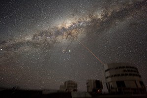
Jansky published his initial findings in December 1932. He reported three sources of radio noise: local thunderstorms, distant thunderstorms, and an unknown source whose azimuth changed gradually each day. This daily pattern initially led Jansky to guess that the Sun was the source. However, as the Sun moved along the ecliptic, additional observations showed the source of the noise did not move with it, ruling out the Sun. These observations showed the static signal repeated every 23h 56m, the length of the sidereal day, indicating it was tied to an area fixed in the sky. Jansky gave an approximate location of the source in the constellation Sagittarius, an area that includes the center of the Milky Way Galaxy. He announced this discovery in 1933.

Radio noise from the heart of the Milky Way — Jansky initially thought the source of radio noise was the Sun, but later realized that it came from the heart of the Milky Way. (Photo is in the optical.)

Jansky published a third paper in 1935 in which he reported radio noise whenever the antenna was pointed in the plane of the Milky Way. He correctly concluded that the emission was from interstellar matter — since stars, including our Sun, emitted much less radio radiation than expected.

Jansky proposed that further developments in radio astronomy would require a dish-shaped antenna to achieve better resolution and better reduction of ambient noise. The antenna would have to be fully steerable like the visible-light telescopes already long in use. Jansky requested resources to pursue these projects but was refused (this was the midst of the Great Depression) and assigned to other duties.

Grote Reber made the first radio map of the sky

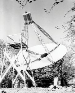
Grote Reber built the first dish antenna radio telescope in 1937. With this 31-foot diameter telescope, Reber mapped the radio structure of our Galaxy, discovered bright sources of radio waves outside our Galaxy, and made the observations that would later help physicists discover non-thermal radiation.
(Credit: NRAO/AUI/NSF)

The developments suggested by Jansky were undertaken by Grote Reber (1911 – 2002). Reber had read Jansky’s work and set about building a 9.5-meter radio telescope on his property in Wheaton, Illinois. His radio telescope looked like the design in use today: a curved dish-shaped reflecting surface and a receiver supported at the prime focus by struts. Reber reasoned that the radio power was a type of light called thermal radiation, i.e., obeyed the laws of blackbody radiation as set down by Max Planck. If so, then the thermal radiation would be brighter – and thus easier to detect – at wavelengths shorter than those investigated by Jansky. Reber’s assumption was incorrect, as we will see later.

[Editors: For the above do we need a drawing of a thermal (blackbody curve) and non-thermal radiation to clarify this point? Yes, but not here]

Jansky’s receiver had been tuned to intercept radio waves at wavelengths of 14.6 m (a frequency of 20 million cycles per second, or 20 MHz) and 10 m (30 MHz). Reber’s first attempt was at the shorter wavelength of 9.1 cm (3300 MHz). The expectation was that it should be a much stronger signal here than at Jansky’s wavelength. However, there was no detection. He then tried 33 cm (910 MHz), again with no success. His third attempt (in 1939), at a wavelength of 1.9 m (160 MHz), resulted in a detection. For the next several years Reber mapped the northern celestial sphere in radio waves, discovering that radio waves emanated most strongly from the plane of the Milky Way, brightest towards the center (Sagittarius) and faintest towards the anti-center (Perseus). He published this work in 1944.

Jansky’s and Reber’s detections suggested the existence of a radio continuum, i.e. radio power emitted over a wide range of wavelengths but not thermal in nature. One source of this continuum is synchrotron radiation. Unlike hot thermal radiation, synchrotron radiation gets brighter at longer wavelengths. Thus synchrotron radiation is often called non-thermal radiation.

The discovery of radio objects

In optical light, Cygnus A appears as an unremarkable starfield. Courtesy NASA/JPL.

Early radio telescopes collected light only from large portions of the sky, too large to discern any detail and often too large to precisely locate the direction to the object. Following the great advances made in antenna technology in WWII, efforts were made to build radio telescopes with the ability to see fine detail. Large radio telescopes were built in the 1950s and 1960s in Australia, the Netherlands, the United States, and England; these countries were the world leaders in radio astronomy for many decades and produced many exciting discoveries.

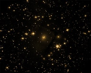
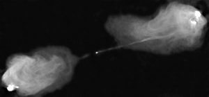
The first discrete and distinct radio source discovered was towards the constellation of Cygnus, thus it was dubbed Cygnus A (Cyg A). Since the resolution of optical telescopes was hugely better than any single radio antenna, astronomers searched for an optical counterpart that could possibly give off that much radio emission. Eventually, a deep investigation using the great telescopes on Mt. Palomar in California revealed a huge and distant galaxy, a type of object today called a radio galaxy.

A radio map of Cygnus A made with the VLA shows an amazing double jet structure. (R. Perley, J. Dreher, & J. Cowen)

Further discoveries followed. Both Taurus A (the Crab Nebula, or Tau A) and Cassiopeia A (Cas A) were found to be the remnants of exploded stars. Eventually, catalogs of radio objects were produced, including the famous Cambridge catalogs. These catalogs are called “1C” for the first Cambridge catalog, “2C” for the second, “3C” for the third, and so on. Objects became known by the catalog in which they appeared. For example, the third Cambridge catalog has 471 entries. Radio source Cygnus A is listed as the 405^th object in that catalog and is thus known as 3C 405. The many catalogs list radio objects such as radio stars, supernova remnants, pulsars, radio galaxies, and quasars.

The discovery of pulsars

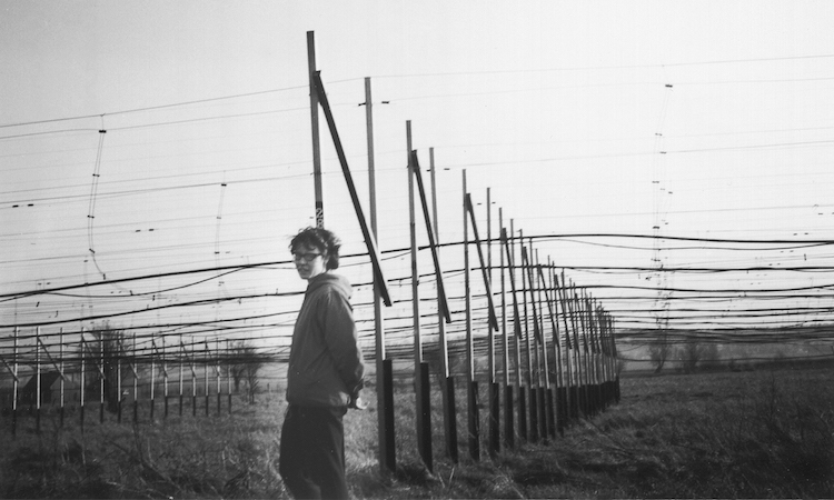
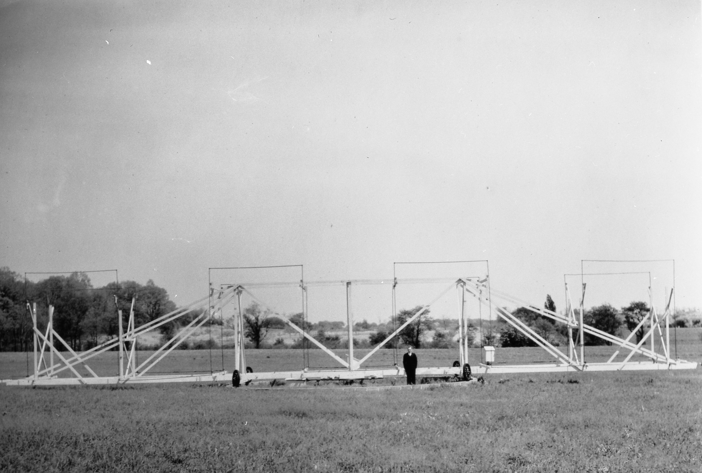
J. Bell by the radio antenna she worked on. — A 1967 photo of Jocelyn Bell by the antenna she used to discover pulsars. (From the collection of J. Bell Burnell)

At Cambridge University, Anthony Hewish (1924 – 2021) undertook a program to study quasars. In 1967 he designed and built a radio telescope with the ability to measure rapid changes in radio brightness (scintillations). He was aided by doctoral students, including Jocelyn Bell (b. 1943). The telescope looks nothing like the classic dish design we think of today; It consisted of 120 miles of wire and cable in a row pattern, which ultimately connected to a receiver. The telescope was a transit telescope, only capable of observing objects as they crossed (transited) a narrow band of the sky centered on its local meridian. As the Earth rotated, celestial radio objects would move across its field of view or “beam”. In this way the telescope surveyed wide bands of the sky each day and the entire sky viewable from its location each week. A strip chart recorder attached to the telescope recorded about 30 meters of paper per day,

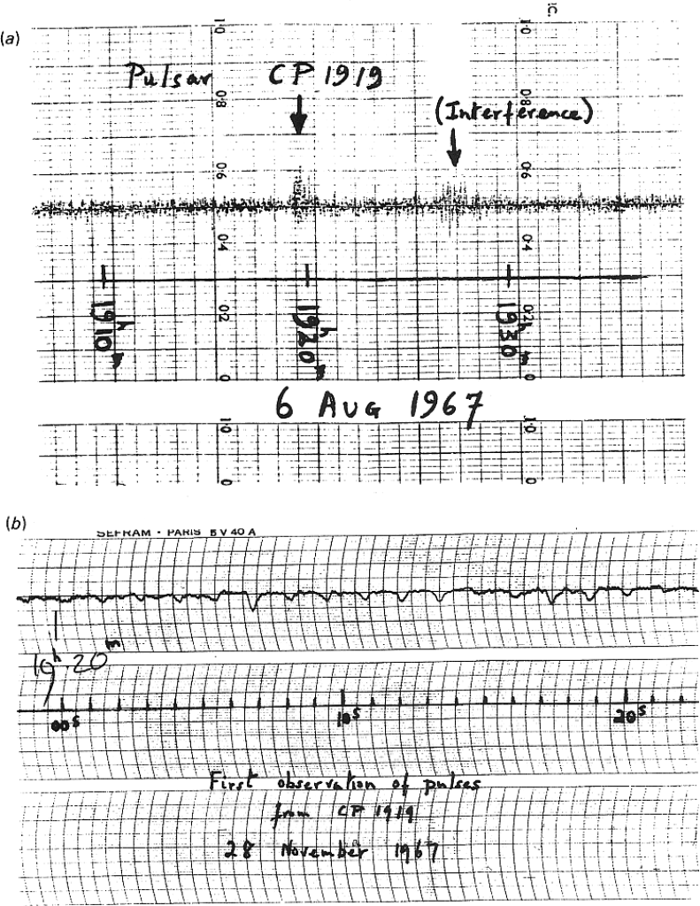
which Bell combed for fluctuating signals that might be scintillating

quasars. Most of these signals, however, represented either terrestrial interference (like the radio noise emitted from the sparks plugs of a car engine), or known types of astronomical radio objects. However, she quickly discovered pulses unlike other forms of interference and reported it to Hewish.

Making detailed observations of her “scruffy” radio source, Bell found it to be a single object fixed on the celestial sphere that appeared to pulse every 1.3 seconds. The signal was so rigidly regular that Bell and Hewish even entertained the fun hypothesis that it might be a signal from an extraterrestrial civilization; they called it “LGM-1” for “Little Green Men”, after the usage in the beloved pulp magazines. With the discovery of more of these objects, the LGM hypothesis seemed unlikely, and they came to be called pulsars. Eventually, LGM-1 became known as PSR B1919 21, because it is located at right ascension 19^h19^m and declination 21º in the Besselian epoch 1950 coordinate system.

The 1974 Nobel Prize in physics was the first Nobel to be given to a discovery in the field of astronomy. It was awarded to Martin Ryle (1918 – 1984) and Anthony Hewish. The citation reads, “for their pioneering research in radio astrophysics: Ryle for his observations and inventions, in particular of the aperture synthesis technique, and Hewish for his decisive role in the discovery of pulsars.” (NobelPrize.org)

The exclusion of Bell was considered by some to be a terrible snub as Bell actually made the discovery, but to others it seemed natural given the leadership role of the professor rather than the student assistant. In 1993, a second physics Nobel prize was awarded in the field of pulsar astronomy, again for a discovery by a graduate student at the observatory working with a professor at the university. By then, the times had changed, and the Nobel Prize was shared between the student and professor. Eventually, Bell would receive lucrative prizes for it, and become knighted by the Queen.

You will be able to repeat Dame Jocelyn’s discovery using essentially the same “transit” method, but using a more modern radio telescope.

Discussion: Observationally Naming New Objects

One question in science is how should we name something new? Our first reaction may be to name it based on what we think it is, physically. However, this can get us in trouble over time.

For example, around 1780 astronomers started seeing objects with angular sizes similar to Jupiter, but much fainter and more diffuse. The objects were named planetary nebulae. Over time, these planetary nebulas have been shown to have absolutely nothing to do with planets. They are not planets, they will not be planets and never were planets. Rather, we now understand them to result from the stellar winds expelled by dying stars.

The confusion this has sown over the years has been a harsh lesson to astronomers. Do not give a wholly new class of objects a name based on what you think they are physically, because you might be wrong. Rather, name new things based on their observational characteristics.

When pulsars were discovered in 1967, by British graduate student Jocelyn Bell and her advisor Anthony Hewish, they first called them little green men mostly as a joke. However, they soon settled on pulsars as an appropriate name. Why? Because they appear to pulse in their radio emission.

At the time, they had multiple hypotheses of what these objects might be, but they also knew that most of those hypotheses must be wrong. So, when they settled on a real name, they wanted to choose a name that would make sense, regardless of what physical model the scientific community would eventually adopt.

How a radio telescope works

[Editors: this section must be reconciled with the What a Radio Antenna Measures section]

As does a reflecting optical telescope, our radio telescope has a parabolic mirror (the dish) to reflect and concentrate radio waves at a point called the prime focus. Here the waves can be picked up by an antenna, and amplified. (Other telescopes may have additional reflectors to focus and concentrate the radio waves into various feedhorns on the dish itself or at other locations.) The signal is then passed to systems that detect and measure it.

At the prime focus, the concentrated electromagnetic waves impinge on a conducting wire called a probe (because it probes the electric field of the impinging electromagnetic wave). Electric fields exert forces on charged particles (electrons) and because electrons are free to move in a conducting wire, variations in the electric field impinging on the wire cause electrons to move in a coordinated response. The wire probe becomes an antenna, a device that turns the tiny variations in the impinging electric field into tiny electric currents in a wire.

Antennas can be made particularly sensitive to a narrow range of wavelengths by adjusting their lengths. [Editors: The coupling can be nicely demonstrated by tuning two wires to the same note, then exciting one – the other will begin to vibrate. maybe imbed a short video or GIF?] The length of each antenna is a simple fraction, such as $\small \frac{1}{4}$ , of the target wavelength. This way, like a guitar string, the arriving electromagnetic wave sets up a standing wave in the antenna. On the 20-meter telescope, two identical probes are lined up linearly such that the total length of the probes is one-half the wavelength of interest. Such an antenna is called a half-wave dipole. [Editors: Standing wave? or couples efficiently)

Often two half-wave dipoles are arranged perpendicular to each other to retrieve useful information about the polarization (orientation) of the impinging electromagnetic wave relative to the dipoles. Each dipole measures the amount of electric field oriented in its direction. Radio light is considered unpolarized if the two different dipoles measure the same electric field strength after all of the correcting calibrations are conducted. Polarization will be discussed in more detail later.

The antenna is connected to the receiver, an electronic device that amplifies, detects, and provides a measure of the intensity of radio signals. In the receiver, each polarization of signal currents is amplified. Amplifiers can strengthen the signal by thousands of times but because they have temperature and radiate as blackbodies, they can introduce significant radio noise. To minimize this noise, amplifiers (as well as the rest of the signal-detection chain) are cooled to temperatures close to absolute zero.

Now that the signal has been amplified, it also needs to be slowed down, so that standard electronics can process it more easily. Therefore, in a step unique to radio, the frequency of the amplified signal is changed by a process called mixing or heterodyning, through which the frequency of the amplified signal is shifted down to the frequency range of the telescope’s detecting electronics. Amazingly, this process is done without losing any of the information in the amplified signal.

An electronic device called a square-law detector converts the signal (which was a measurement of current in a wire) into a measurement of power. This conversion involves electronically squaring the signal. [Current is directly proportional to voltage and the square of voltage is directly proportional to power.] We say a signal is “detected” once this conversion is made.

Many additional electronic signal conditioning operations can take place within the receiver/detector, including analog to digital conversion, narrowband filtering, Fourier analysis, extraction of polarization information, and signal integration and averaging. Once completed, the detected signal is available for external analysis. When you view your data you will have two independent signals, one from each of these dipoles.

Problem #0:

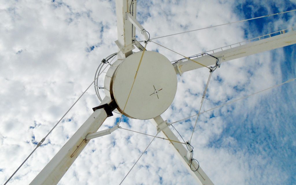
Secondary reflector showing feeds — A picture of the prime focus of a VLA 25-meter antenna located in Magdalena, NM, USA.
(Photo: Stan Converse)

Shown at the right is an image of the prime focus of a 25-meter Jansky Very Large Array (VLA) radio telescope. There are two sets of linear feeds, one set (the cross) tuned for $\lambda = 90$ cm radiation and the four wires on the outside to pick up $\lambda = 400$ cm radiation. Each pair of feeds (vertical and horizontal) are connected to a low-noise amplifier—one for each polarization. The flat surface is a 2.35-meter diameter reflector to focus higher frequency radio waves to a cold receiver at the Cassegrain focus.

The cross is formed by two dipoles, one for each polarization.
(a) By measuring the picture, estimate the length of each dipole.
(b) Find the ratio of each wire length to the wavelength of sensitivity. This should be approximately a simple ratio, such as 1:2, or 1:4. If it is a 1:2 ratio, we say it is a half-wave dipole antenna, and similarly, if it is a 1:4 ratio, we say it is a quarter-wave dipole antenna. Which is it?

Observe a High S/N Radio Pulsar by Transit

Chart recorder traces of the original detection of a pulsar. (Image: Jocelyn Bell Burnell and Anthony Hewish)

[Editors: this is a quick one observation exercise which demonstrates the detection by Bell and demonstrates the pulsed signals. Also, it might be useful to have a video showing the telescope moving in a daisy since we cannot notify students when their observation runs]

There are a few pulsars accessible from Green Bank that have a high enough signal to noise ratio to be clearly observed with a modest radio telescope. In this brief exercise you will recreate Jocelyn Bell’s discovery by observing one of these pulsars. You will observe this pulsar using a 20-meter class radio telescope and look for the regular pulses characteristic of a pulsar in the recorded data.

The Hewish telescope Bell used was only capable of viewing sources as they transited the local meridian, an event which happens once every 23h 56m. The telescope was electronically pointed at an area of the sky, and the pulsar “drifted” across its beam. It would not be seen again for another sidereal day.

Since our telescope can be made to move, we can do this much more quickly: we will “drift” the telescope beam across the pulsar instead of waiting for the pulsar “drift” across the telescope beam.

Setting up your observation

The way we will accomplish our “transit” observation is by having the telescope move across the pulsar as part of a daisy scan. In this type of scan, the telescope beam crosses the center of the target multiple times while also observing areas in a pattern that looks like a daisy. Pulsars suitable for this type of observation are listed in the following table. The “Difficulty Level” is an indication of how likely you are to get good results on your first try.

Table #1: High S/N Pulsar Candidates to Observe by Transit
	B1950 Name	Right Ascension (hh:mm:ss) J2000	Declination (dd:mm:ss) J2000	Difficulty Level
1	PSR B0329+54	03:32:59.3	54:34:45.0	Easy
2	PSR 0833-45	08:35:20.7	-45:10:35.2	Lightly Challenging
3	PSR B0950+08	09:53:09.2	07:55:36.4	Lightly Challenging

To Do This:

Login to https://skynet.unc.edu/, then My Observatory and then Radio Observing.
Click “ Add New Observation”.
Enter the J2000 RA and Dec of the pulsar you choose from the table above.
Adjust:
- Min Target Elevation – within 10 degrees of its peak on the Target Visibility Chart. For PSR B0833-45, set the Min Target Elevation to 4 degrees.
- Min sun separation at least 2 degrees
Receiver Settings
- Low Resolution
- HI filter
- 1024 channels
- Do not select Pulsar Mode
Path Type: Daisy
Radius (arcmin): 60 to 120^[2]
Number of Petals: 4
Duration: 320s^[3]
Integration time: 0.002 s

What to Expect:

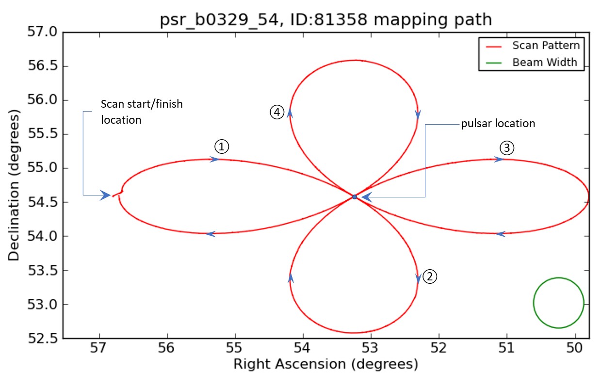
When your observation runs, the telescope will point itself at a position to the side of your target pulsar (at an RA later than the pulsar RA by about twice the Radius you entered but at the correct Dec). It will then move in a daisy pattern as illustrated in the figure below, first along path ①, then along paths ②, ③ and ④, finishing at the original start point. In the process the beam will cross the pulsar four times. The pulsar will be in the beam for a time dependent on your observation Duration and Radius settings.

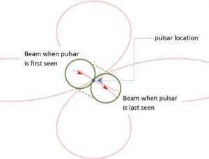Location of the beam when it can "see" the pulsar

A typical 4-petal daisy mapping path.

Movement of the telescope beam across the pulsar on its first crossing.

The continuum data collected for each polarization will be plotted on a Power vs Time graph. Two traces will be visible, one red, one green. These two sets of data are collected automatically by the telescope and allow astronomers to determine whether and how the radio signal is polarized. One polarization trace may have better S/N than the other: if so, use it.

[Editors: Insert a plot of a non-pulsating source in a 4-petal daisy as an illustration? 3C147 is a good one…]

Question: For a 360s observation, at what approximate time should you expect to first see the center of your pulsar signal appear in the continuum data? At what other times should it appear? [Note: When looking for your pulsar signals, add 10s to the times you just calculated to account for a calibration signal injected at the beginning (and end) of each observation.]

Question: Longer-term undulations in Power level not due to the pulsar may be observed. Suggest a source for these slow undulations.

Question: By correlating the scan path with the continuum data can you suggest one or more locations for the undulation-producing source(s)?

Live Continuum mode.

When your observation completes, your data can be accessed by the following steps:

Go to your Skynet radio observations
Click on your observation number to go to the observation page.
Under Observation Data click on the link: National Radio Astronomy Observatory – Green Bank website
Click on the Live Continuum link

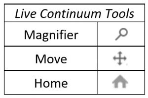When the Live Continuum page opens you can explore your data interactively using the three tools provided: the magnifying glass, the move tool, and the undo (home) tool.

The Magnifier tool allows you to zoom in on the plotted data in a unique way: You draw a rectangular box over the area you want to zoom in on, and it resizes and redraws your data in such a way that the rectangle is converted to the viewing window. For example, suppose you draw a perfect square… the resizing/redrawing just zooms in to that area, equally magnifying in the x- and y-directions. Now suppose you draw a rectangle three times wider (x-direction) than it is tall (y-direction): the resizing/redrawing then magnifies the y-direction by a factor of three relative to what it does to the x-direction in the process of creating the new viewing window. This stretching if the y-data makes any pulses more noticeable.

The Move tool allows you to move the plot around in the viewing window by clicking and dragging with your mouse. In this mode you can also zoom in and out using the mouse wheel.

The Home tool undoes all operations and returns you to the original plot.

Problem: Drag the plot until the pulses are close to the time scale and zoom in on the pulses themselves. Reposition as necessary. Make a guess at the pulsar’s period. Compare it to the known period.

What have you accomplished?

You have recreated Bell’s initial pulsar discovery with a high S/N pulsar. The only thing you did differently is you “drifted” the telescope beam across the pulsar instead of waiting for the pulsar “drift” across the telescope beam. That and the fact that you knew pulsars exist and where to find them – a big difference!

What a Radio Antenna Measures

The fundamental difference between a radio telescope and an optical telescope is that the frequency of the the radio light is low enough that it can be measured as a signal rather than as total energy.

[Editors: This section will deal with noise, the many temperatures and noise reduction; influence of integration time; etc.]

If you played the signal output from a radio telescope on your radio, it would sound like static, which is often referred to as white noise. Radio astronomers measure the average intensity of this static. The more data that we collect and add up, or average, the better our signal to noise becomes, so long as we are averaging measurements of the same thing. For example, say we observe an object that does not change with time for 30 seconds, average the data, and find a signal to noise ratio of 3. Then if we average data from the same object collected for 120 seconds, we would find a signal to noise ratio of 6. If we collect 4 times more data, our signal to noise ratio increases by a factor of 2. We can write this as a proportionality between the signal to noise ratio $\frac{S}{N}$ and the total observation duration, τ.

(1) $\begin{equation*} \frac{( \frac{S}{N} )_2}{( \frac{S}{N} )_1 } \propto \sqrt{\frac{\tau_2}{\tau_1} \end{equation*}$

This can be more tricky, however, when observing a pulsar, because it changes quickly with time. In particular, it does no good to average together times when the pulsar is on and off. You will address this problem by only averaging data that are in phase, resulting in a folded light curve.

Due to random motion of charged particles (electrons), all objects have temperature and radiate light. Such radiation is called thermal radiation or blackbody radiation. Since it is due to the random motion of charged particles, it is always unpolarized, unless it is observed after having been reflected. For example, polarized sunglasses help block glare on your windshield or the surface of a lake, but direct sunlight is unpolarized. Since hotter objects radiate more thermal radiation at all wavelengths than cooler objects, radio telescopes often measure the intensity of a source in equivalent temperature units. For example, say you point a radio telescope at some large area of the sky with a temperature of 256 K, that area would have a brightness temperature of $T_B = 256 K$ . The brightness temperature is an intrinsic property of the radio source; if the source is a true blackbody it is the physical temperature of the source.

The brightness temperature can never be directly measured for several reasons. First, the beam of the telescope may be larger or smaller than the radio source. What the telescope sees is the average of all emissions in the beam. Second, what the telescope sees depends on the size of the dish. Further, all the components of our radio telescope and its environment have thermal energy that contaminates the signal. Rather, we measure the signal plus the thermal noise, which when expressed as a temperature is called the antenna temperature $\left( T_A \right)$ . The antenna temperature has nothing to do with the physical temperature of the antenna. The antenna temperature is the temperature of a blackbody placed in front of the antenna that would give off the same amount of radio signal that telescope receives, or, said another way, the temperature of the sky + environment averaged over the telescope beam.

Often most of the noise is due to the temperature of the first amplifier, located inside the receiver, so it makes sense to express the total noise in the system also as temperature, which is called the system temperature $\left( T_S \right)$ . The system temperature s the total noise added by everything except the source we want to observe. Finally, we can express this as:

(2) $\begin{equation*} T_A = T_B + T_S \end{equation*}$

Where $T_A$ is what we measure, and $T_B$ is what we are interested in.

In practice, we usually measure the system temperature ( $T_S$ ) by pointing at a nearby area of the sky which doesn’t include a radio source (much like subtracting off the background sky in optical astronomical photometry). You do not need to do this for observing pulsars, however, because they turn on and off. Since it is off more often than it is on, a running median does a nice job of characterizing the system temperature as a slowly changing function of time.

If your source object happens to be both thermal and extended (i.e. it’s angular size is larger than the field of view), then the brightness temperature ( $T_B$ ) is the object’s physical temperature. If, on the other hand, it is a point source (i.e. it is smaller than the field of view), then the brightness temperature is proportional to the flux density, and can be best found by observing an astronomical calibration source just before, and just after, the observation.

Objects that have temperature constantly emit blackbody radiation including at radio frequencies. While a light detector on a room-temperature optical telescope housed in a closed, darkened dome would see nothing, a room-temperature radio telescope within the same darkened dome would be flooded by radio emissions. These emissions come from the dome, the earth, and all components of the telescope itself. If the dome were opened, it would also see radio emissions from the atmosphere and from space. This radiation is called system noise and is always present. Even in the best of circumstances, the signal we are interested in may be only a percent or so of the total signal received and must be extracted from it ~~by differentiation~~. With pulsar observations, this can be accomplished by averaging the total signal over an integration time and subtracting that average from the total signal. This works because the system noise is approximately constant over short time periods, whereas the pulsar signal is not. Subtracting the average signal from the total signal reduces the noise leaving the pulses (increases the signal-to-noise ratio). Of course, this process is not perfect because the system noise is only approximately constant, and the averaged signal includes the signal of interest as well as the system noise.

Key Takeaways:

Radio antennas measure static, called white noise.
The signal to noise ratio of a constant source increases with a longer observation.
Radio antennas measure two perpendicular polarizations.
All thermal sources emit unpolarized radiation.
The system temperature $T_S$ is a measurement of the noise.
The antenna temperature $T_A$ is what the antenna measures.
The brightness temperature $T_B$ is the temperature your source would have, if it were an extended thermal source.
$T_A = T_S + T_B$ .

Observe a High S/N Pulsar by Tracking

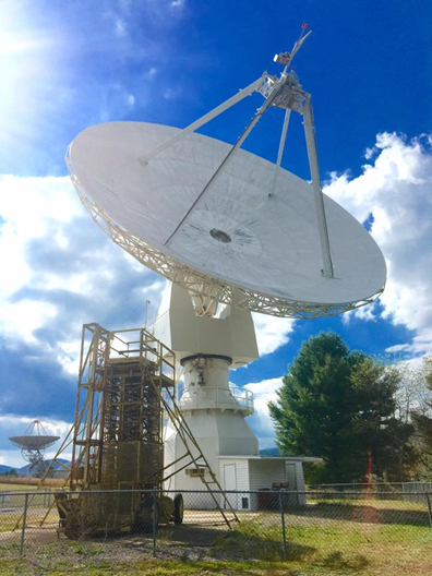
Skynet's 20 meter telescope at the Green Bank Observatory — The 20-meter radio telescope at the Green Bank Observatory is available for your use.
(Photo: Green Bank Observatory)

Previously you detected high S/N pulsars by the transit method. This method does not work for low S/N pulsars because the pulses are hidden in the background noise. We must use longer observations to collect more data and mathematical methods to pull the signal out of the noise. We will first learn this method using our high S/N pulsars as preparation for observing low S/N pulsars. In this exercise, you will again observe these pulsars using a 20-meter radio telescope, but aim the telescope directly at the pulsar and track the pulsar as it moves with the celestial sphere. You will collect sixty seconds of data, and investigate it using the mathematical tools built into Skynet’s plotting software. Ultimately you will determine the period of the pulses, and produce what is called a folded light curve.

Submitting your observations

First observe a pulsar that is easy to detect, such as PSR B0329 54. Once you understand the process, repeat it for another more challenging pulsar.

Table #2: High S/N Pulsar Candidates to Observe by Tracking
	B1950 Name	Right Ascension (hh:mm:ss) J2000	Declination (dd:mm:ss) J2000	Difficulty Level
1	PSR B0329+54	03:32:59.3	54:34:45.0	Easy
2	PSR B2021+51	20:22:49.8	51:54:50.2	Lightly Challenging
3	PSR B1133+16	11:36:03.0	15:51:15.5	Lightly Challenging
4	PSR B1919+21	19:21:44.8	21:53:02.2	Lightly Challenging
5	PSR B0950+08	09:53:09.2	07:55:36.4	Challenging
6	PSR B1929+10	19:32:14.0	10:59:33.3	More Challenging

Link to Video: How To Observe a Known Pulsar Using Skynet — Video: How To Observe a Known Pulsar Using Skynet

[Editors: B0833-45, an 89ms pulsar, is an easy target, good sonification, but you sure won’t be able to count beats! so…. I’ve left it out. ]

To do this:

Login to https://skynet.unc.edu/, then My Observatory and then Radio Observing.
Click “ Add New Observation”
Enter the J2000 RA and Dec of the pulsar you choose
Adjust:
- Min target elevation at least 30 degrees.
- Min sun separation at least 2 degrees
Receiver Settings
- Low Resolution
- HI filter
- 1024 channels
- Do not select Pulsar Mode
Track
Integration time 0.02 s
Observation Duration 60 s
Repeat 0

Notes: This is a real telescope, and sometimes a pulsar does not show up due to atmospheric or interstellar medium distortions on the line of sight. Also, sometimes the antenna works better than at other times. And, most importantly, it is easy to be confused by a terrestrial radio source (called a birdie in the jargon). Therefore, you will need to look at your data soon after your observation is completed, and see if it makes sense. If it does not, submit another observation of the same source. The higher the difficulty level in the table, the more likely you will need multiple attempts to observe your source.

Discussion: Naming Conventions

Astronomers name individual objects using naming conventions, which are rules that each new discoverer follow.

For example, every new solar system planet must be named after some mythological god or goddess. Similarly, moons of the planet are named after characters associated with the god. For example, Galileo wanted to name the moons of Jupiter after his patron, but was later overruled and they are named after various lovers of Zeus. The only exception are the moons of Uranus, as William Herschel also wanted to name his new planet after his patron, and the moons after characters in two British plays. He was overruled as to the planet’s name, but his naming convention for Uranus’s moons stuck. Sometimes new discoveries become catalogued before their physical nature is known. For example, the brightest radio source in the constellation of Cassiopeia is called Cassiopeia A. These names stuck for the most bright radio objects, but were later superseded by the Third Cambridge Catalogue of Radio Sources, which gave each a number. More recent naming conventions often include the coordinates of the object. Pulsars, for example, are named after their Right Ascension and Declination in the sky. However, due to the precession of the equinoxes coordinates change over long periods of time. In the mid 20th century, astronomers reported coordinates fixed in the year 1950, but in the late 20th century we switched to fixing to the year 2000. This means that a few very bright pulsars retain their B1950 coordinate names, while all others now use a J2000 coordinate name. For example, in the case of the pulsar PSR B0329+54, it is located at a B1950 celestial coordinates RA=03^h29^m11^s, and Dec= 54º24’39”. However in J2000 coordinates, it is located at RA=03^h32^m59^s, and Dec= 54º34’45”, so is also called PSR J0332+5434. You may ask, how do we know when the same object has multiple names? In practice, for objects in our Galaxy we look them up in the SIMBAD Astronomical Database based in Europe, and for extragalactic objects we use the NASA Extragalactic Database based in North America.

Analyzing your data

Once your observations have been completed, which might be quite soon since radio telescopes can observe both during the day and night, you may investigate and download your data. For radio astronomy, your Skynet results page will link to another page at the Green Bank Observatory. It is on that page that you can look at, and download, your light curve data.

To get your data:

Go back to your Skynet radio observations
Click on your observation number to go to the observation page.
Click on the link to your observation from the Green Bank Observatory.
Download your calibrated continuum data as a text file. This file contains the antenna temperature in Kelvin as function of time in seconds.
Now open the Skynet Plotting Tool (skynet.unc.edu/astro101L/graph)
Select Pulsar, and then upload your data file.
Click on Sonify and listen to the pulsar’s signal. [Editors: Is there a way to get a moving cursor such as is standard in Audacity to show where the playback is in the graph?]

Now you should hear, and see on the graph, the signal as a function of time. If you can hear a repeating pattern along with the noise, then you can measure the period. If you cannot, you may want to reobserve your object, especially when you chose a more challenging pulsar to observe.

Link to Video: How To Analyze Pulsar Data Using the Skynet Plotting Tool — Video: How To Analyze Pulsar Data Using the Skynet Plotting Tool

Once you have data where you can hear a beat over the static, then do the following:

Count the number of the beats you hear in 30 seconds. Like music, you are looking for the tempo, so if you do not hear a particular beat, count it anyway. Write this down.
Calculate the period by dividing the number of beats into the time. Again, write this down.
Click on Periodogram, and set the period range around your measured period.
This will calculate a power spectrum, which is the power received as a function of time period.
The peak period from each polarization (remember the perpendicular dipoles?) “should” agree with each other and your measured period. They will not quite agree, which will allow you to estimate the error in your measured period.
Next make a folded light curve using the period that you just found. This averages data that are the same phase, to show a light curve over one or two periods. Again, you should have two independent curves: one per polarization.
Measure the time that the pulse is on. This is called the pulse width. [Editors: FWHM or what? Does it matter?]
Click on sonify again, to listen to your data. It should sound less noisy, and more regular, but otherwise similar to what you heard before.
Now, change the period slightly, and repeat this process over and over, until your light curves show the narrowest pulses and your are satisfied that you have the correct period. [Editors: Need to expand on this process of iteration – it moves 1 decimal place at a time. It would be nice to show in the video]

Now that you have two folded light curves, one for each perpendicular polarization, you can ask whether the incoming radio waves are polarized. Recall that if they are unpolarized, the signal will be the same for each polarization. Therefore, their light curves should match, and when you sonify your data the left and right channels should sound the same. The catch, however, is that it is possible that one polarization channel may amplify the signal more than the other, making an unpolarized signal appear to be polarized. Therefore, to test for polarization, you will need to calibrate one channel to match the other as best as you can. If you try very hard to get rid of any polarization, but it is still impossible through calibration, then the source emits polarized light.

To calibrate the polarizations, do the following:

Click on Polarization Calibration: Show Difference
This subtracts one polarization from the other, and plots this difference for you.
Adjust the calibration until the two polarizations match as best as you can. [Editors: Are the two polarizations calibrated equally?]
Can you get the two polarization light curves to match perfectly? If you can, you are observing unpolarized light. If you cannot, you are observing polarized light.
Click on Sonify again, to listen for a difference in your two stereo channels. Since there are two polarizations, and computers play stereo sound, each stereo channel will play a different polarization. You might hear a difference, but you might not, depending on your pulsar, your headphones, and your hearing.

[Editors: Should we talk about the “washing” sound they will hear due to the peaks arriving at different times?]

Your Observational Results:

What is the name, and location in the sky, of your pulsar?
What is the measured period of your pulsar?
What is the width of the pulse in seconds?
About what is the brightness temperature of the pulses. [Editors: why would they know how to get the brightness temperature?]
Is the light polarized or unpolarized? How do you know?

Physically Interpreting Your Results

Fundamentally the goal of astronomy is to understand the nature of the universe. This does not just mean what objects look like, but rather what they are physically. As of now, you have come up with a number of observational results, which are the clues we need to piece together the mystery of what these pulsars really are.

As does any puzzle solver, astronomers ask many “what if” questions, and then eventually settle on those hypotheses that explain existing and future observations. Astronomers call this modeling, but one could also call it reasoning by analogy.

The lighthouse model

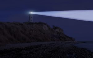
Lighthouse with a cone of light — A lighthouse emits a cone of light, as seen in this picture taken on a foggy night. However, a distant ship on a clear night simply sees it blink on and off.
(photo credit: Flash Alexander)

What could possibly appear to turn on, and off, at a regular interval? We may imagine that there is someone turning a light on and off, which is of course why Bell & Hewish first called pulsars little green men. However, the reason little green men was a joke, was that they knew there had to be a natural explanation. In nature objects spin and orbit, but they rarely blink on and off. So, what is something that appears to turn on and off, but is really rotating?

Consider a lighthouse in the middle of a dark, but not foggy, night. A distant ship will only see the lighthouse when the light is pointing at it, so it will appear to blink. A sailor on the ship could even figure out the opening angle of the light cone by setting up a ratio with a full circle:

$\frac{\theta}{360\deg} = \frac{\rm pulse \, width}{\rm pulse \, period}.$

Problem #1: Using the lighthouse model, estimate the opening angle of the pulsar you observed.

The lighthouse model is an example of a good toy model, in that it expresses the correct essence of a physical solution, but at the same time it leaves out many details. The wonderful thing about a good toy model, however, is that you can see it in your mind’s eye.

The lighthouse model also leads to a whole bunch of new questions, such as:

What is spinning?
Why is the beam collimated?

We will be able to answer these questions, but first we need to understand what is producing the light in the first place.

Discussion: Toy Models in Science

Scientific models can get very complicated very quickly, and it is quite easy for scientists to spend years refining a model in exhaustive detail.

Hopefully one has the right basic idea before working out the details. To avoid wasting too much time on completely wrong models, scientist first come up with simplistic models to test. These are called toy models, so everyone knows that there are many details that are left out. If a toy model cannot explain the observations in general, it probably cannot after the details are worked out. On the other hand, just because a toy model successfully explains the observations does not mean it is necessarily correct. Sometime competing toy models explain the same basic observations, and astronomers then must carefully plan future observations that will distinguish between them.

Thermal radiation

Fundamentally electromagnetic radiation is created when a charged particle, such as an electron, accelerates. Since electrons are less massive, they accelerate more than protons when acted on by the same force, so they are the ones that radiate the most light.

Electrons can accelerate for a number of different reasons, some of which are directly related to their temperature, which sets the electrons into random motion. These are called thermal processes, and the resulting light is called thermal radiation. Hallmarks of thermal radiation are:

The light is unpolarized.
The intensity peaks when the thermal energy approximately equals the photon energy $\left( k \, T \approx h \, f \right)$ . Given the low energy of radio waves, thermal sources increase in intensity as the observed frequency increases.

If, however, an electron accelerates for reasons having little to do with its temperature, such as being accelerated by an electromagnetic field, this is called non-thermal radiation. This radiation may, or may not, be polarized, and where its intensity peaks have little to do with its temperature.

There are many forms of natural non-thermal radiation, and almost all of them have to do with charged particles that, for some reason other than temperature, are moving close to the speed of light. Sometimes these high-energy particles collide with something else and release their excess energy. These collisional mechanisms may appear quite similar to thermal emission, in that they emit mostly high-energy photons and are unpolarized.

Fundamental Question #1:

Is the emission you observed from PSR B0329 54 thermal emission? Clearly explain your answer from your observational evidence.

Non-Thermal radiation

Non-thermal radiation simply means that the radiation is not thermal. Just because some radio waves are both unpolarized and the intensity peaks at a very short wavelength, does not necessarily mean that it is thermal, but it is almost always thermal in practice.

However, the opposite must be true. If light is polarized, it must be non-thermal. Similarly, if the radio intensity increases with wavelength, it also must be non-thermal. So, what kind of natural source could produce such a thing?

First, we will consider everyday sources of radio waves, such as communication antennas. The electrons in these emit radio waves because the driving electric field wiggles the electrons back and forth in unison, thus emitting radio waves at that same frequency. The question, therefore, is what natural process could possibly accelerate electrons collectively? The most likely possibility could be that the electrons interact with electromagnetic fields.

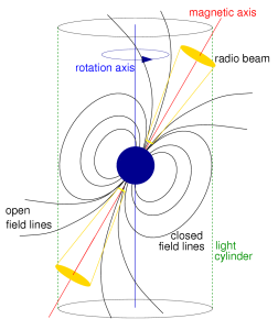
Polarization and magnetic fields

Electrons move in circles perpendicular to strong magnetic fields, but they can flow freely parallel to them, so they follow helical paths.

[Editors: I would like to replace the figure]

Unlike electric fields, magnetic fields do not exert forces on stationary charged particles. However, when a charged particle moves at an angle to a magnetic field it does experience a force. This force is perpendicular to both the velocity of the charge and the magnetic field and causes the charge to spiral around the magnetic field lines. Because the particle will accelerate in the direction of the force (perpendicular to the magnetic field), but be free to flow parallel to the magnetic field:

Charged particles can flow freely parallel to the magnetic field.
Charged particles cannot flow perpendicular to the magnetic field.
Electrons will emit radio waves polarized perpendicular to the magnetic field.

A nearby example of this is the northern, or southern, lights. In the case of the aurora, charged particles in the solar wind interact with the earth’s magnetic field and become deflected along the Earth’s magnetic field toward the earth’s magnetic poles. We see aurora when the solar wind particles interact with the Earth’s atmosphere.

Perhaps the non-thermal radiation coming from a pulsar has to do with the interaction between a wind of charged particles and a strong magnetic field.

Discussion: Matter and Antimatter

The universe is electrically net neutral, and the only two common charged particles are the electron and the proton, so they must exist in equal numbers. An electron is much less massive than a proton. Since the acceleration a particle experiences in the presence of a force is inversely proportional to mass, electrons accelerate much more and therefore give off the bulk of the radiation we observe, especially in the radio part of the electromagnetic spectrum.

However, for every particle found in nature, there is a corresponding anti-particle, which has the same mass but opposite charge. For example, the antimatter equivalent of an electron is called the positron. When an electron and a positron meet, they attract each other and annihilate, producing two neutral particles of light called photons.

The opposite of annihilation can also happen. If there is enough excess energy, then electrons and positrons can be produced in equal numbers simply from the energy available. This is called electron-positron pair production.

Since there appear to be so many electrons in the pulsar winds, but relatively little mass, most astronomers think that about half of these “electrons” are actually positrons, as there is clearly plenty of excess energy to produce them in pairs. Once produced, these positrons would act just like electrons (except they would be forced in the opposite direction) and when they accelerate they would radiate just like electrons. From a distance, we would not know the difference.

A spinning magnet is like a power plant

So far we have made two physical conclusions:

Since the light is somewhat polarized, there probably are strong magnetic fields near the emission source.

Next let us consider a power plant that makes electricity. One way they work is by spinning a magnet inside a coil of wire. The spinning magnet induces a voltage across the wire coil, producing the power you consume. Here we have something spinning, and it seems we have a magnetic field because we have polarized radio emission, so what if we have a spinning magnet like a power generator?

In a power generator with a spinning magnet, the peak-to-peak AC voltage across each loop of the coil is the radius of the loop times the magnetic field times the relative speed. You can calculate the surface speed of the pulsar from your period measurement, as a function of the radius. First, we know that the circumference of a circle is simply π times the diameter, or circumference = 2πR, therefore:

(3) $\begin{equation*} v = \frac{\rm circumference}{\rm period} = \frac{2 \pi R}{P} \, , \end{equation*}$

so in terms of your measured period, the radius of the pulsar (R), and the magnetic field (B), the voltage (V) induced by the pulsar would be:

$V = R \times B \times v = R \times B \times \left( \frac{2 \pi R}{P} \right) = \frac{2 \pi \, R^2 \, B }{P}$

So, depending on the strength of the magnetic field, this voltage may be much greater than the 120 V peak-to-peak in North American houses.

[Editors: Should we point out that you don’t need a wire to have a voltage difference in space?]

As an example, let’s now calculate the equivalent voltage the Earth creates. Recall that the radius of the Earth is 6 400 km and its period is 23h56m = 86 000 s. The SI unit of magnetic field is the Tesla, named after famous electrical engineer Nicola Tesla. At the equator, the Earth’s magnetic field is about 30 microtesla or 0.000 03 tesla. Therefore the Earth’s voltage would be:

(4) $\begin{equation*} V_{\oplus} = \frac{2 \pi \, R_{\oplus}^2 \, B_{\oplus} }{P_{\oplus}} = \frac{2 \pi \, \left( 6\,400 {\rm m} \right)^2 \, \left( 0.000\,03 {\rm T} \right) } {\left( 86\,000 {\rm s} \right)} = 0.1 {\rm V} \end{equation*}$

As you can see, this is not enough to matter here on Earth. However, if the magnetic field of the Earth were much bigger, or if the Earth spun faster, it would act more like the dynamo inside of everyday power plants, much less the largest voltages that we can create on Earth.

[Editors: Not sure what the preceding sentence or the following sentence is supposed to say]

[Editors: Should we say here that we will revisit this voltage calculation later for pulsars?]

Schematic of a model of a pulsar as a small spinning magnet. — A spinning magnet provides a good physical model of a pulsar. In this drawing, the white loops represent the magnetic field lines and the blue cone represents the beam of radio waves. (Made by Mysid in Inkscape, based on en:Image:Pulsar schematic.jpg by Roy Smits., CC BY-SA 3.0, https://commons.wikimedia.org/w/index.php?curid=2612701)

Since we are doing observational astronomy, the important thing is what we can observe, and that the lighthouse toy model seems to work well. So, perhaps, the spinning pulsar provides enough voltage to provide an outward wind of charged particles, and the magnetic field then collimates them into a pair of jets at the poles. Like the aurora, but backward, with the wind coming from the pulsar. Since the magnetic field is both strong and curved, the electrons must accelerate and produce electromagnetic radiation. When those same electrons are moving close to the speed of light (i.e. relativistic), the radiation is beamed in the direction of the velocity — along the direction of the jet. Therefore, a combination of a high induced voltage and a curved magnetic field could explain why a beam of radio waves could emanate from the pulsar’s magnetic poles, and if the magnetic axis is not aligned with the rotational axis the beam will act like a lighthouse.

Key Takeaways:

A spinning magnet induces a voltage, like in an electric power plant.

This high voltage can produce a strong wind of charged particles emanating away from the pulsar.

This wind will follow the magnetic field, so it will be beamed along the magnetic axis.

The magnetic field is slightly curved away from the poles, which accelerates the electrons, making it radiate linearly polarized radio waves.

This refinement of the Lighthouse Model can explain your observational results so far.

What can a pulsation period tell us?

Now you know, because you observed it using data from your radio observation, that the object you observed appears to pulse on a regular basis with a pulsation period that we will call P. This is, of course, why they were called pulsars (see box). But what might a pulsar be physically? That is the fascinating question.

First let us imagine that a pulsar is some object that is spinning on its axis, in much the same way that Earth does. Let us begin, therefore, with our first physical assumption:

Physical Assumption #1:
The pulsation period represents the rotation period of some spherical object.

With your observed pulsation period, and this assumption, what can we learn?

The goal of this section is to develop a physical model of a pulsar using only your observational data, and astronomical evidence known to Bell and Hewish in the late 1960s. Remember, science is a process, not a result!

A pulsar must be smaller than its light cylinder

Light Cylinder illustration — The light cylinder is an imaginary cylinder coaxial with the star’s rotation axis where rotation speeds equal the speed of light (Figure source: NRAO)

Once we assume that the pulsation period is the rotation period of an object, we realize that it must be spinning very fast. However, nothing can travel faster than the speed of light, including the surface of pulsar. The place where its surface would be moving at the speed of light, is called the light cylinder. Here we calculate the radius of the light cylinder, and use it to put a hard upper limit on the pulsar radius.

By way of analogy, let us first calculate the surface speed of the Earth.

We will do this by dividing the distance the equator travels in one sidereal day by the Earth’s rotational period. The Earth’s polar circumference, by the original definition of the meter, is exactly 40 000 km, and its equatorial circumference is slightly more (40 075 km). The Earth’s rotation period is: 23^h56^m = 1 436 min = 86 160 seconds. Thus the speed of Earth’s equator is 0.465 kilometers per second. (e.g. One km/s is about the top speed of the fastest fighter jet.)

Now let’s apply exactly the same technique to finding the speed of the surface of the round object that we are assuming rotates, which we are calling a pulsar. The astute reader will now protest, “we do not know the circumference of the pulsar, so how can we find the surface speed?” What we will actually do, rather, is find the speed as a function of the radius of the pulsar, with the goal of narrowing down what the radius could be based on the object’s equatorial speed.

Let us now call R the radius of the pulsar, v its equatorial surface speed, and of course P the period that you already measured. Now we can write the equatorial surface speed, $v$ , as in equation 3:

$\begin{equation*} v = \frac{\rm circumference}{\rm period} = \frac{2 \pi R}{P} \end{equation*}$

The catch, however, is that we know neither v nor R. However, we can put some constraints on what the velocity, v, could be. To begin with, we know that v must be less than the speed of light, because according to Einstein’s Theory of Relativity nothing can move faster than light. Mathematically we can write this as: $v < c$ , where c is the speed of light. Now substituting for the velocity into equation 3, and solving for the radius, we find that
$v = \frac{2 \pi R}{P} <c$ and so $R < \frac{c P}{2 \pi}$ .

Key Takeaway:
Since the equatorial surface speed must be less than the speed of light, the radius must be less than the radius of the light cylinder, which is defined as where the rotation speed would be the speed of light. Mathematically this is expressed as:
$R < \frac{c P}{2 \pi}$ , where R is the radius of the pulsar, P is its period of rotation, and c is the speed of light.

For example, if the pulsar period were one second, then the radius must be given by the inequality:

$R < \frac{c P}{2 \pi}$ so $R < \frac{ ( 300 000 {\rm km/s} ) (1 s )}{2 \pi}$

Therefore: $R < 50 000 \, {\rm km}$ , which is about the radius of Saturn.

Notice that we have not calculated that a pulsar with a period of one second is about the size of Saturn, but rather that is cannot be as big as Saturn. It, very well, could be much smaller!

Problem #2: Use this speed of light inequality, and the rotation period that you measured, to find the radius of the light cylinder. Argue that this is a hard upper limit on the radius of the pulsar.

Would a pulsar flatten itself by spinning too fast?

Next, we will make another assumption to narrow the pulsar size even down more. Recall that the Gas Giant planets in our solar system are oblate due to their rotation about an axis. The same thing happens to all astronomical objects that are spinning, unless their mass is great enough to hold them together. To understand this, we must calculate two things: the surface gravity of the object and the acceleration of its surface. Only if the surface gravity, g, is greater than the centripetal acceleration of the surface, $a$ , then the object will be able to hold itself together. This leads us to our next physical assumption.

Physical Assumption #2:
The equatorial surface acceleration must be less than the surface gravity. $\left( a < g \right)$

Next we recall that velocity is simply the circumference divided by the period, so from introductory physics, the centripetal acceleration can be written in terms of the radius and the period as:

(5) $\begin{equation*} a = \frac{v^2}{R} = \frac{ \left( \frac{2 \pi R}{P} \right)^2}{R} = \frac{ 4 \pi^2 R}{P^2} \end{equation*}$

Let’s again use the Earth as an example. We know that the earth’s equatorial radius is 6 378 km and its period is one sidereal day (23h 56m = 86 160 s), so the centripetal acceleration at the equator is:

$a_{\oplus} = \frac{ 4 \pi^2 R}{P^2} = \frac{\rm 4 \pi^2 (6\,378 m) }{\rm (83\,160 s)^2} = 0.034 \frac{\rm m}{\rm s^2}$

We know that its surface gravity is $g_{\oplus} = 9.8 \frac{\rm m}{\rm s^2}$ , which is much bigger than the centripetal acceleration. This is good, because we know the earth exists.

Problem #3: Calculate the Earth’s centripetal acceleration, if it rotated with the period you measured for the pulsar. How many times greater is this than that the earth’s surface gravity?

Could a pulsar be a spinning white dwarf star?

From the last problem you showed that if your pulsar were the size and mass of the earth, it would fling itself apart. Therefore, it must have a much greater surface gravity than the earth, and, in turn, a much greater mass. Since the sun has a much greater mass than the earth, perhaps the pulsar has approximately the mass of the sun, but the size of the earth?

There exists a common class of objects, whose mass is similar to the sun’s mass and radius similar to the earth’s radius. These are called White Dwarf stars, which you observed in the unit on HR diagrams. Let us now calculate the surface gravity, g, of a typical White Dwarf star using Newton’s law of gravity:

(6) $\begin{equation*} g = \frac{G \, M}{R^2} \end{equation*}$

where G is Newton’s Constant, M is the mass of object, and R is its radius.

Since this applies to any round object, including Earth, this is most easily solved in ratio to the earth. Here we use the subscript “WD” to stand for the white dwarf and $\oplus$ for the earth.

$\frac{g_{WD}}{g_{\oplus}} =\frac{\frac{G \, M_{WD}}{R_{WD}^2}}{\frac{G \, M_{\oplus}}{R_{\oplus}^2}} = \frac{\frac{M_{WD}}{M_{\oplus}}}{\left( \frac{R_{WD}}{R_{\oplus}} \right) ^2}$

Notice that constants always cancel when solving problems in ratio to a known quantity.

In this case, we are assuming that the mass of the object is about one solar mass, which is 300 000 times greater than the mass of the earth. However, we are also assuming the radius is the same as the earth, so we can now plug in these two ratios (300 000:1 and 1:1) to estimate the surface gravity of a white dwarf star:

$\frac{g_{WD}}{g_{\oplus}} = \frac{300\,000}{\left( 1 \right) ^2} = 300\,000$

So, an object the same size as the earth, but with a mass the same as the sun, would have a surface gravity 300 000 times greater than we experience here on Earth.

Problem #4: Based on the measured period, and your solution to Problem #3, does it make sense for your pulsar to be a spinning white dwarf? Explain quantitatively using the acceleration inequality $a<g$ .

How small must a pulsar be, if it had the mass of the Sun?

In the prior sections, we notice that stars make up a great deal of objects in our Galaxy. And in the last problem, you showed that a white dwarf start would fling itself apart if it were spinning anywhere near the rate of your pulsar. Now we will calculate a new upper-limit on the size of a pulsar, if its mass were the same as the sun. We will, now, set up the acceleration inequality, with the equations 5 and 6.

(7) $\begin{equation*} \left( a = \frac{ 4 \pi^2 R}{P^2} \right) < \left( g = \frac{G \, M}{R^2} \right ) \end{equation*}$

Now, we can solve for an upper limit to the radius of the pulsar:

$\begin{equation*} \left( \frac{ 4 \pi^2 R}{P^2} \right) &< \left(\frac{G \, M}{R^2} \right) \, \, \rightarrow \, \, \left( { 4 \pi^2 R^3} \right) &< \left({G \, M \, P^2} \right) \, \, \rightarrow \, \, { R^3} &< \left(\frac{G \, M \, P^2}{4 \pi^2} \right ) \end{equation*}$

Therefore:

(8) $\begin{equation*} R &< \sqrt[3]{\left(\frac{G \, M \, P^2}{4 \pi^2} \right ) } \end{equation*}$

Notice something interesting: this follows exactly the same mathematical form as the orbital radius of a hypothetical satellite orbing just above the surface.

Now, for example, we can write the radius of a one solar mass pulsar with a period of one second as:

$\begin{align*} R &< \sqrt[3]{ \frac{ \left( 6.67 \times 10^{-11} {\rm \frac{m^3}{kg \, s^2}} \right) \, \left( 1.99 \times 10^{30} {\rm kg} \right) \, \left( 1 \rm s \right)^2 }{4 \pi^2} \right) } \\ R &< 1 \, 500 \, 000 {\rm m} \end{align*}$

This is using the consistent SI system of units, based on the meter, kilogram, and second. To put this into context, this means that a solar mass pulsar, with a period of 1 second, must be smaller than 1500 km, which is smaller than the moon. Again, it may be much smaller than the moon.

Problem #5: What is the maximum radius that a solar mass object could have, and also rotate with the pulsar period that you measured?

Discussion: Falsifiable Hypotheses in Science

What distinguishes science from non-scientific subjects? Why do scientists eventually reach agreement, even if after heated debates? Ultimately it is because scientific questions are answered through the process of hypothesis testing, which is both a way to investigate the natural world and a way to resolve differences.

We are not interested in measurement for measurement sake, but rather as a tool to understand the natural world. Ultimately, we are interested in the physical nature of faraway objects, such as pulsars, and so we brainstorm about what they might be. For example, we asked if your observed pulsar could possibly a spinning planet, but we soon found that it would fling itself apart because it was spinning to fast. Then we asked if it could be a white dwarf star, and again we found that it too would fling itself apart. In these cases, we considered a hypothesis, but ultimately ruled it out based on physical principles and observational data.

In particular, Scientific Hypotheses must be falsifiable, meaning that it would be quite easy, in principle, to nullify them. All one has to do is conduct an observation that contradicts the hypothesis. If there are no observations one can possibly conduct to test an idea, then the idea has no scientific meaning. It might be fascinating, and it might be true, but how do we know?

Falsifiable hypotheses work well to resolve disagreements. Rather than arguing, two people can agree to conduct future observations that could falsify the hypothesis. If observationalists try very hard to nullify a theory, and still fail, then over time the theory becomes accepted.

Notice that in this class, you are the observationalist, and your job is to nullify one hypothesis after another. If you work hard, and still fail to do so, maybe you will start believing that the theory actually represents reality.

The density of a pulsar

When we are interested in what something is made of, we often find its density by dividing the volume into the mass. Clearly, lead is more dense than water, which in turn is more dense than air. Once we calculate the density, we can begin to ask about the material that makes it up.

In your case, once you have measured the period of the pulsar, then you found an upper limit on the radius. However, to do so, you had to make the gross assumption that its mass was the same as that of the sun. This was plausible, but by no means well justified — and definitely not measured. Since small things are denser than big things, we expect to find a lower limit on the density, D..

To see this mathematically, we will substitute in the volume of a sphere to the density equation, so:

$D = \frac{\rm mass}{\rm volume} = \frac{M}{V} =\frac{M}{\frac{4 \pi}{3} R^3} .$

Now we are tempted to substitute in the radius R from our inequality above, but since that is an inequality it makes more mathematical sense to solve for the radius in the equality above.

$D = \frac{M}{\frac{4 \pi}{3} R^3} \rightarrow R^3 = \frac{M}{\frac{4 \pi}{3} D} \rightarrow R = \sqrt[3]{\frac{M}{\frac{4 \pi}{3} D}}$

Now, we can write our inequality as:

$R = \sqrt[3]{\frac{M}{\frac{4 \pi}{3} D}} < \sqrt[3]{\left(\frac{G \, M \, P^2}{4 \pi^2} \right ) } .$

Now we can cube both sides, and inspect the following equation:

$\frac{M}{\frac{4 \pi}{3} D} < \frac{G \, M \, P^2}{4 \pi^2} .$

Notice something totally amazing! By dividing both sides by the mass, they cancel out. What this means physically is that we can solve for the density lower limit, knowing only the pulsar period! Finally we can write:

$\frac{1}{\frac{1}{3} D} < \frac{G \, P^2}{\pi} \rightarrow \frac{1}{3} D > \frac{\pi}{G \, P^2}$

Notice how we flipped the inequality sign when we took the reciprocal of both sides. Finally, multiplying by three, we obtain:

(9) $\begin{equation*} D > \frac{3 \pi}{G \, P^2} . \end{equation*}$

Again, this simple result is important, as it gives us a lower limit on the density simply as a function of period, which it the first thing measured for any pulsar. We do not have to make a guess of either the mass or the radius..

For example, a pulsar with a period of 1 second would have a density of:

$D > \frac{3 \pi}{\left( 6.67 \times 10^{-11} \frac{\rm m^3}{\rm kg \, s^2} \right) \left( 1 \, \rm s \right)^2 } .$

Which comes out to be $D > 1.4 \times 10^{11} \rm{\frac{kg}{m^3} }$ .

For comparison, the density of water is 1000 kg/m³, and the density of Earth is 5 500 kg/m³, with its core having a density of about 10 000 kg/m³. Thus, the density of a one-second pulsar must be greater than ten million times the density of Earth’s core, or else it would fling itself apart. And, as before, remember that this in an inequality, so it actually could be much more dense than this!

Problem #6: Calculate the minimum density your pulsar could possibly have, without it spinning itself apart?

Problem #7: Assume a typical white dwarf star, with a mass about that of the sun, and a size about that of the Earth. a) Calculate this star’s density in SI units, and b) express your pulsar’s density inequality in ratio to this typical white dwarf.

What material could a pulsar possibly be made of?

As of now, you have investigated the idea that a pulsar could be a spinning planet, and found that it would be spinning much too fast to hold itself together. Then you asked if it could be a spinning white dwarf star, and again you found that it would be spinning too fast. So, what could possibly be this dense? We know it is much denser than anything we have ever experienced.

The discovery of the atomic nucleus

This leads us back in history to a series of experiments conducted between 1908 and 1913 in Ernest Rutherford’s laboratory at the University of Manchester, where Hans Geiger and Earnest Marsden performed an experiment where they shot positively charged alpha particles into very thin (0.6 µm) gold foil. They had expected them to pass right through, which is exactly what happed to most of them—but a very small fraction (about 1 in 8000) came crashing back at them.

From this they concluded that matter is mostly made up of empty space, with the mass concentrated into a very small, and dense, region that they called the nucleus. Knowing the fraction of the particles that bounced back allowed them to work out an upper limit on the size of the nucleus, and in turn its density.

At this time, in 1909, the diameter of an atom had been known to be about 10^-10 meters for over 40 years, based on work by Johan Loschmidt^[4]in 1865 that measured the size of air molecules. Therefore, based on Geiger and Marsden’s work, we can estimate the size of interaction between an alpha particle and a gold nucleus.

We will start by letting the fraction of the alpha particles that bounce off of the nucleus to be $f_{\rm bounce} = \frac{1}{1800}$ , as they observed. Then we realize that the shadow cast by a circle is given by the cross-sectional area, so the chance that a nucleus is struck must be the ratio of the cross-sectional area of the nucleus to that of the whole atom, or:

$f_{\rm bounce} = \frac{A_{\rm neucleus}}{A_{\rm atom}} = \frac{\pi R^2_{\rm neucleus}}{\pi R^2_{\rm atom}} = \left( \frac{R_{\rm neucleus}}{R_{\rm atom}} \right)^2$

Now we can solve for the effective nuclear radius, as:

$R_{\rm neucleus} = R_{\rm atom} \sqrt{f_{\rm bounce}}$

Next we will think about how the nucleus interacts with an alpha particle. Given that it has a positive charge, and so do alpha particles, they must repel even when not touching. Therefore this is the effective radius for the interaction between these positive particles, which means that the actual nuclear radius can be much smaller than this, but it may not be bigger. Finally we obtain this inequality:

(10) $\begin{equation*} R_{\rm neucleus} < R_{\rm atom} \sqrt{f_{\rm bounce}} \end{equation*}$

Problem #8: Based on the gold foil experiment, and Loschmidt’s estimated diameter of an atom, find the radius of the gold nucleus. Express your answer as an inequality.

Nuclear physics greatly took off during the 1930s, and then accelerated during the Second World War, with the making of the atomic bomb. After the war, it really flourished, as there was a great deal of new research funding, especially in America. Therefore, by the 1960s, when Bell and Hewish discovered pulsars, the size and the mass of atomic nuclei were quite well known. Now we know that all atomic nuclei have about the same density, which is about 2 ✕ 10¹⁷ kg/m³, regardless of the atom in which they reside.

Problem #9: Imagine that a pulsar actually has the same density as a typical atomic nucleus. Calculate the size of a one solar mass pulsar. Does this seem reasonable given what you have already discovered.

The existence of neutron stars

In the last few problems, you showed that your pulsar must be denser than any known object, except for the nucleus of atoms. So, perhaps, a pulsar is simply a really large atomic nucleus. While this idea agrees with our observational data, it has one significant flaw: there are no elements heavier than Uranium found in nature. The problem has to do with the proton, and the very strong electric force between charged particles. The more protons one packs together, the stronger the repulsion force pushing them apart. Therefore, it should be impossible to make a giant nucleus with a radius you found in Problem #9. What could possibly resolve this problem?

Going back to 1920, enough work had been done to understand that sometimes atoms of the same element have different masses. These are called isotopes, and it led Rutherford to the hunch that each nucleus contained both positive and neutral massive particles, called protons and neutrons. The atom’s chemical properties are governed by the number of protons, but the mass is given by the total number of protons and neutrons. This led to experimentalists searching for these neutral particles, which James Chadwick of the Cavendish Laboratory at Cambridge University succeeded in doing in 1932^[5] As with all discoveries, however, it was really not one person, but each study builds on prior ones. For example, his work built on that of others, such as Irène & Frédéric Joliot, whom he cites. And, of course, much of the work in nuclear physics was pioneered by Irène’s parents, Marie and Pierre Curie.

The question for Bell and Hewish in the 1960s, therefore, was not whether there could be a huge atomic nucleus, but whether there could be a star made of only neutrons. Since they have no net charge, neutrons should be able to be packed together tightly, so the hypothesis makes sense. But how could such a thing come about? How does one pack together a solar mass of only neutrons, when matter is made up of neutrons, protons, and electrons in approximate equal numbers. Shouldn’t anything made from normal matter, however it is made, be made of an approximately equal mix of protons, electrons, and neutrons?

The solution came in the form of a particular type of radioactive decay called electron capture, or more specifically K-capture, which was first predicted in 1934 by the Italian physicist Gian-Carlo Wick, and then observed three years later by the American physicists Luis Alverez.^[6] In some proton-rich nuclei, an inner electron (a K-shell electron) combines with a nuclear proton to produce a neutron and a neutrino, which reduces the total potential energy of the atom. Now the question is this: could it ever be energetically favorable to make a giant ball of neutrons?

In a 1934 paper on a different topic, astronomers Walter Baade and Fritz Zwicky gave the following answer to this question:

With all reserve we advance the view that a super-nova represents the transition of an ordinary star into a neutron star, consisting mainly of neutrons. Such a star may possess a very small radius and an extremely high density. As neutrons can be packed much more closely than ordinary nuclei and electrons, the “gravitational packing” energy in a cold neutron star may become very large, and, under certain circumstances, may far exceed the ordinary nuclear packing fractions. A neutron star would therefore represent the most stable configuration of matter as such.^[7]

We now understand that a pulsar is a neutron star that we can see rotate by observing it in the radio part of the electromagnetic spectrum.

Key Takeaways:

Neutron stars are objects that are about the mass of a star, but made of only neutrons.

Pulsars are spinning neutron stars.

Neutrons are little magnets

There are a number of properties of fundamental particles, which include mass, charge, and magnetic moment. The neutron has about the mass of a proton, zero charge, but about the same magnetic moment as a proton (the electron’s is much bigger).

The magnetic moment is the fundamental strength of a magnet. Unlike charge and mass, magnetic moment is a vector. For example, in a permanent magnet the magnetic moments all point the same direction, but in an unmagnetized material the magnetic moments point every which way.

Now imagine that somehow, probably because of the magnetic field of the original star, all of the magnetic moments in a neutron star aligned in the same direction. Then the total magnetic moment would simply be the sum of magnetic moments of all of the neutrons. If that were the case, the magnetic field near the poles of a neutron star would be about a trillion teslas. If, on the other hand the neutrons were randomly oriented, then there would be no net magnetic moment. So, in math notation we have: $B < 10^{12} \rm T$ . The magnetic field may be much smaller, but this is such a huge number that one can see how a pulsar can be a incredibly powerful dynamo.

Problem #10:
Use equation 4 to calculate an inequality for the voltage produced by your pulsar, assuming it is a spinning neutron star.

Problem #11: The mass energy of an electron is the same as its kinetic energy would be if it were accelerated by a voltage of 500 MV ( $5 \times 10^8 \rm V$ ), so we say it has a mass of 500 MeV (mega electron volts).

Using your result from problem #11, write down an inequality for the ratio of the kinetic energy to the mass energy of an electron in the pulsar jet.

If this is greater than 1, we say the electron is relativistic. Discuss whether the spinning neutron star can explain the existence of relativistic electrons in pulsar winds.

Observing Low S/N Pulsars by Tracking

Next you will observe pulsars that are significantly dimmer than the one you have already observed. This is significantly more difficult, because each pulse is no brighter than the noise. In radio astronomy lingo, the system temperature is greater than the brightness temperature ( $T_S > T_B$ ). How do we observe these dim pulsars?

Recall taking optical images, where the noise was often greater than the signal. Up to a point, with a long enough exposure the signal can become greater than the noise, because the signal to noise ratio was proportional to the square root of the exposure time ( $S/N \propto \sqrt{t}$ ), where t is the exposure time. In other cases, the S/N ratio can be greatly improved by aligning and stacking short exposures.

The problem with a radio pulsar, however, is that you found the signal as a function of time. If you increase the integration time, it will beat down the noise—but it will also smear out our pulse signal.

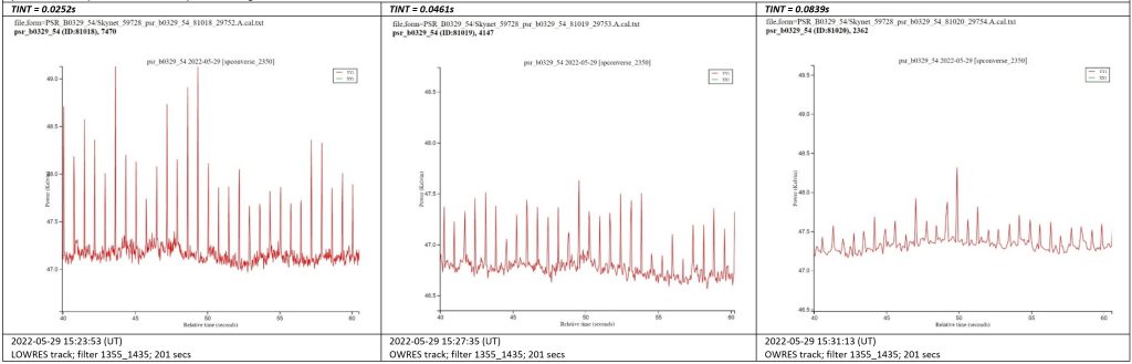
Effect of integration time on signal to noise ratio — Three sequential 180s observations of B0329+54 showing the effect of Integration Time on both noise and signal. Longer integration times reduce the noise, but also reduce the signal because the integration window is not in phase with the pulses and thus the pulses average out as well.

The solution is to sample quickly (short integration time), but increase the Observation Duration. Because pulsar signals brighten and dim minute to minute due to interactions with the interstellar medium (ISM), a longer observation will have more instances where the signal is present and thus amenable to mathematical methods. Your light curve will look like noise, until you fold and bin your data (think align and stack). Then, you can make a folded light curve. There is a catch, however. In order to fold and bin your data, you must be able to determine or already know the period.

As it turns out, there are a number of fast algorithms for finding the period of a signal underneath the noise, and the Skynet Periodogram uses one of them. The results, however, will be less clean than in the high S/N pulsar case, because the pulsar signal only a tiny fraction of the noise signal. In practice, the very first time an astronomer observes a pulsar finding the observed period can be quite difficult. On the other hand, subsequent observers know the prior result, so they know the approximate period. This helps them improve measurements and distinguish pulsars from noise sources.

In this part, you will need to pick a low S/N pulsar, and complete the same analysis as you did before. You will submit a Skynet observation, download your data, listen for a pulse pattern (Can you pick it our?), run the periodogram, create a folded light curve, and finally listen for a pulse pattern again (can you hear me now?). The primary goal of this part is to understand how noise averages out when independent data are averaged together.

Table #3: Low S/N Pulsar Candidates to Observe by Tracking
	B1950 Name	Right Ascension (hh:mm:ss) J2000	Declination (dd:mm:ss) J2000	Period (s)	Difficulty Level
1	PSR B0628-28	06:30:49.3	-28:34:42.2	1.244418596	Very Challenging
2	PSR B0736-40	07:38:32.2	-40:42:39.4	0.374920736	Very Challenging
3	PSR B0835-41	08:37:21.1	-41:35:14.5	0.751625423	Very Challenging
4	PSR B1933+16	19:35:47.7	16:16:40.0	0.358738411	More Challenging
5	PSR B0740-28	07:42:49.0	-28:22:43.5	0.166762292	Most Challenging
6	PSR B1641-45	16:44:49.2	-45:59:09.7	0.455078202	Most Challenging
7	PSR B1749-28	17:52:58.7	-28:06:33.9	0.562557636	Most Challenging
8	PSR B2045-16	20:48:35.7	-16:16:46.9	1.961572304	Most Challenging

Observing Faster Pulsars

[Note to editors: We have found only one “fast” pulsar that we can detect in 3 minutes or less in pulsar mode, namely B0833-45, an 89ms high S/N pulsar. Detecting Crab (33ms) requires 30 minutes of observation in pulsar mode… see observation 81479. Do we want to change the emphasis here from fast pulsars to just pulsar mode?]

You may now wonder how do we observe pulsars that are faster than the sampling rate? The answer is that we cannot, but we can increase our sampling rate. The problem with this, however, is that we produce too much very noisy data to process easily.

On the other hand, what if we observe a known pulsar, and have an idea of what the observed period will be beforehand? Then it is possible to analyze the data on the fly with a dedicated fast computer—called a pulsar backend. Our radio telescope has the option to route the data through the pulsar backend, which will find the period and fold the light curve for you.

In short, this pulsar backend simply does what you did for the slower low S/N pulsar, but it does it much more quickly. ^[8]

In this section, you will observe a faster pulsar. ~~of your choice~~, however now click pulsar mode. When this box is checked, your signal is routed through the pulsar backend.

[Editors: We have found only one “fast” pulsar that we can detect in 3 minutes or less in pulsar mode, namely B0833-45, an 89ms high S/N pulsar detected easily even by transit. Detecting Crab (33ms) requires 30 minutes of observation in pulsar mode… see observation 81479. Do we want to change the emphasis here from fast pulsars to just pulsar mode?]

You can then then upload the folded light curve, graph it, and listen to the sound.

Next, revisit all of the problems you were assigned for the high S/N pulsar, and make the same calculations using your fast pulsar.

see: Keohane, J.W. & Foy, J.P., (2019), An Introduction to Classical Electrodynamics, ISBN: 978-1-949942-00-2, https://maricourt.press ↵
You must guarantee that the telescope beam moves completely off the target. With that accomplished, the smaller the Radius the longer the pulsar is in the beam.. See figures. ↵
320s or 400s; a multiple of 8 is desirable. The greater the Duration, the longer the pulsar is in the beam. See figures. ↵
Loschmidt, Johann, On the Size of Air Molecules, Proc. of the Academy of Science of Vienna, (1865) vol 52, p.395-413, Translation in the Journal of Chemical Education for October 1995, vol 72, No. 10, p. 870-875. (see: https://www.chemteam.info/Chem-History/Loschmidt-1865.html) ↵
Chadwick, J., Possible Existence of a Neutron, Nature 129, 312 (1932) (see https://web.mit.edu/22.54/resources/Chadwick.pdf) ↵
Over 40 years later, Luis and his son Walter, a geologist, would publish the hypothesis that the mass extinction of the Cretaceous dinosaurs had been caused by the impact of an asteroid. ↵
Baade, W. and Zwicky, F., Cosmic Rays from Super-Novae, Proceedings of the National Academy of Sciences, 1934, 20 (5) 259-263 https://doi.org/10.1073/pnas.20.5.259 ↵
In order to observe very fast pulsars, the pulsar backend also must take into account a few other things, such as how light changes speed with frequency when traveling through a medium, a phenomenon called dispersion. ↵

License

The Multiwavelength Universe Copyright © by Jonathan Keohane; Daryl Janzen; David Moffett; Michael Allen; Kalee Tock; Aaron LaCluyze; Stanley Converse; Daniel Reichart; Megan Dubay; Colin Wallace; Elijah Hayes; Gloria Brown SImmons; Jeff Regester; John Torian; Joshua Haislip; Kate Meredith; Logan Selph; Matthew Fleenor; Michael Fitzgerald; Rielly Castle; and Ruide Fu. All Rights Reserved.