4
Joel Bruneau and Clinton Mahoney
Learning Objectives
- Define the consumer choice problem
- Solve a consumer choice problem with the typical utility function
- Solve a consumer choice problem with utility function for perfect complements and perfect substitutes
Module 4: Consumer Choice
The Policy Question: Hybrid Car Purchase Tax Credit—Is it the Best Choice to Reduce Fuel Consumption and Carbon Emissions?
The U.S. government offered a tax credit toward the purchase of hybrid cars with the goal of reducing the amount of carbon emissions U.S. cars produce annually. We are using the tools of microeconomic consumer theory to study this policy and assess the effectiveness of this policy in reducing emissions.
We are now very close to being able to predict how consumers will change their driving and gasoline purchases in response to a government tax credit on hybrid cars. As we will see, this is simply a specific example of the general question we first raised in Module 1 of how to predict consumer behavior when prices or incomes change. For our policy example and in general, we address this question by combining the budget constraint with the concept of preferences and utility maximization. All of consumer theory in economics is based on the premise that each person will try to do his or her best given the money they have and the prices of the goods and services they like. This is what we mean by utility maximization – choosing the affordable bundle of goods and services that returns the highest utility.
Think about a consumer who goes grocery shopping. There are many ways to fill a shopping basket – ending up with many different possible bundles of goods. This module is concerned with how each consumer picks the best affordable. As we will see shortly, consumers think about the income they have, and the relative prices of all the possible goods they could buy, and then choose among all of the possible bundle combinations that their budget can support.
Exploring the Policy Question
What is your prediction about how consumers’ driving and gasoline purchasing behavior will change when their income increases or decreases? When the price of gasoline increases or decreases? What implications will these behavior changes have for the hybrid car tax credit policy?
4.1 The consumer choice problem: maximizing utility
LO1: Define the consumer choice problem.
4.2 Solving the consumer choice problem
LO2: Solve a consumer choice problem with the typical utility function.
4.3 Corner solutions and kinked indifference curves
LO3: Solve a consumer choice problem with utility function for perfect complements and perfect substitutes.
4.1 The consumer choice problem: maximizing utility
LO1: Define the consumer choice problem.
What is the consumer’s optimal choice among competing bundles? This question summarizes the consumer choice problem. To resolve this problem, we can combine our understanding of the budget constraint and preferences as represented by utility functions. The budget constraint describes all of the bundles the consumer could possibly choose. The utility function describes the consumer’s preferences and relative level of satisfaction from the consumption of bundles. We put these two pieces together by answering the question: Among all the bundles the consumer could possibly choose, which one returns the highest level of utility?
Conceptually, we are overlaying the indifference curve map on the budget constraint and looking for the point or points of intersection, as in Figure 4.1. Recall that there can be more than one indifference curve for bundles of goods A and B. The goal for solving the consumer choice problem is to get on the highest indifference curve – the curve that is the farthest to the upper right – while also satisfying the budget constraint. The highest indifference curve – the one that represents the highest level of utility or satisfaction – is the one that just touches the budget line at a single point. It is not possible to get on a higher indifference curve given the budget constraint, and though it is possible to get on a lower one, doing so necessarily means a lower level of utility or satisfaction.
Figure 4.1 Indifference curve on the budget constraint
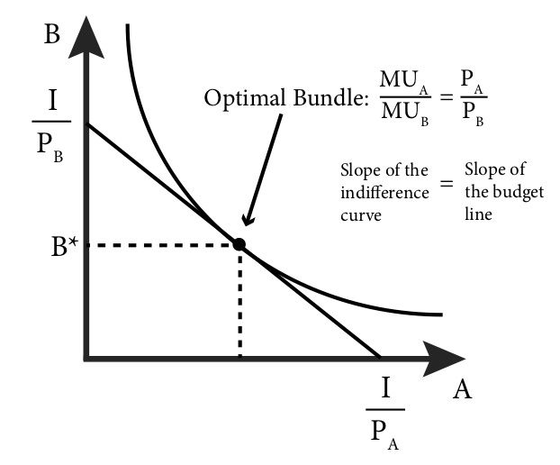
Figure 4.1 summarizes the solution to the consumer choice problem: The consumer should pick the one bundle that returns the highest level of utility while also satisfying the budget constraint. This graph also shows us the two fundamental conditions that represent the solution to the consumer choice problem:
1. The consumer’s optimal choice is on the budget line itself, not inside the budget constraint. This is why we can focus on the line rather than the whole set of affordable bundles.
2. At the optimal choice, the indifference curve just touches the budget line and so at this one point they have exactly the same slope.
This second condition has a significant intuitive interpretation. Recall that the slope of the indifference curve is the marginal rate of substitution(MRS) – the rate at which the consumer is willing to trade off one good for the other and remain just as well off. Recall also that the slope of the budget line is the economic rate of substitution (ERS) – the rate at which the consumer is able to trade one good for the other at current prices. What figure 4.1 shows is that at the optimal choice these two things must equal. But why?
Consider a point, like point 1 in Figure 4.2, where the indifference curve intersects the budget line. Here, the MRS is greater than the ERS is absolute value. The MRS tells us the amount of good B the consumer is willing to give up to get one more unit of good A and remain just as satisfied. In this case, the ERS tells us how much of B a consumer must give up in exchange for one unit of A in the marketplace. Here, the consumer is willing to give up a lot of B to get a little more A and remain just as satisfied, but the ERS indicates that the consumer does not have to give up that much of B to get the same amount of A. So it must be the case that if the consumer trades some of B for A in the market he or she will be better off. In other words, a consumer who moves down along the budget line will be on a higher indifference curve.
Figure 4.2 Budget line with 3 indifference curves.
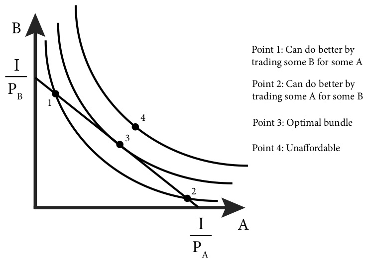
So, the graph of the budget line and indifference curves illustrates the two conditions that define the consumer’s optimal choice:
(1)
and
(2)
(note that the negative signs cancel)
With these two conditions, we can solve the consumer choice problem mathematically.
Note that the MRS=ERS condition can be rearranged to:
Economists sometimes call this the ‘equal bang for the buck’ condition because the equation indicates that at the optimal choice the consumer must be getting exactly the same marginal utility per dollar from the consumption of goods A and B. Why? Think of a case where these two goods are not equal. If you’re at a pizza parlor eating slices of pizza and bowls of salad, suppose that:
This equation indicates that marginal utility per dollar of pizza is less than the marginal utility per dollar of salad at your current level of consumption. You cannot optimize your utility. Why not?
For simplicity let’s assume the price of both a slice of pizza and a small salad is exactly $1, so:
Now, let’s take $1 away from pizza and spend it instead on salad. You lose the marginal utility of that last slice of pizza, but you gain the marginal utility of one more serving of salad. From the condition above, we know that total utility must have increased since:
We also know that marginal utility for a normal preference diminishes when you consume more of a good, and therefore increases when you consume less, . Therefore, the marginal utility of pizza will increase and the marginal utility of salad will decrease, getting you closer to equality. As long as this condition is not met (as long as there is an inequality), a consumer can always make these types of trades to become better off.
4.2 Solving the consumer choice problem
LO2: Solve a consumer choice problem with the typical utility function
Formally, the consumer’s optimal choice problem looks like this:
As we discussed in the Section 4.1, the second line of this problem (the ‘subject to’ part) is the budget constraint. Since we have the more-is-better assumption, the consumer will always spend all of his or her budget on goods A and B. So, we can rewrite the consumer choice problem as:
Let’s use the Cobb-Douglas utility function and solve this problem analytically. Our problem is now:
(4.3)
To solve this problem, we will apply what we know from Section 4.1: At the optimal solution, we have two conditions, MRS=ERS, and we are on the budget line.
MRS=ERS in this case requires that we find the marginal utility of bundles A and B. This requires determining the partial derivative of the utility function for good A and then for good B.
The MRS is the ratio of the two marginal utilities:
The ERS is the ratio of the prices:
Putting these two equations together gives us:
The second part of the consumer choice problem, the budget constraint (that we are on the budget line or the ‘subject to’ part), is straightforward:
At this point, solving the problem is a matter of simple algebra. We have two equations with two unknowns, good A and good B. We can solve these equations by repeated substitution: solve equation (4.4) for good A or B and substitute the result into equation (4.5).
If we solve (4.4) for bundle B, we get:
Substituting into (4.5) gives us:
Simplifying this equation gives us:
Solving for A, we get:
(4.9)
Plugging this equation into (4.6) gives us:
Simplifying this equation gives us the solution for good B:
(4.10)
Remember that the prices, the income, and the parameter values for alpha and beta are all just numbers that are given. Therefore, these solutions for goods A and B are simply a specific amount of both – one specific bundle of A and B consumption that is the very best choice a consumer has among all the possible choices.
Equations 4.9 and 4.10 are the demand functions for goods A and B, respectively. Demand functions are mathematical functions that describe the relationship between quantity demanded and prices, income and other things that affect purchase decisions. We can use these demand functions to predict what will happen to the consumption of both goods when prices and incomes change. From the demand functions, it is easy to predict that increases in the price of the good will lead to lower consumption and increases in income will lead to greater consumption. We will return to the examination of these demand functions in the next module.
4.3 Corner solutions and kinked indifference curves
LO3: Solve a consumer choice problem with utility function for perfect complements and perfect substitutes.
So far, we have considered the optimal consumption bundle for a consumer who has ‘well- behaved’ preferences, meaning that he or she has indifference curves that are smooth, curved in, and not touching the vertical or horizontal axes. The optimal choice for these well-behaved preferences is characterized by the MRS=ERS. The solution to the consumer choice problem with these preferences is always an interior solution: a utility maximizing bundle that has a positive amount of both goods.
But we know that there are other relatively common preference types, such as perfect complements and perfect substitutes, that have indifference curves that are shaped differently. The solution to the consumer choice problem for these preferences types cannot be characterized by the MRS=ERS condition.
As we saw in Module 2, perfect complements have indifference curves that are kinked at 90-degree angles, and perfect substitutes have indifference curves that are straight lines that begin and end on the axes. For both perfect complements and perfect substitutes the solution to the consumer choice problem is the one consumption bundle that puts the consumer on the highest indifference curve possible. But in both cases, this does not have the tangency condition of the MRS equaling the ERS.
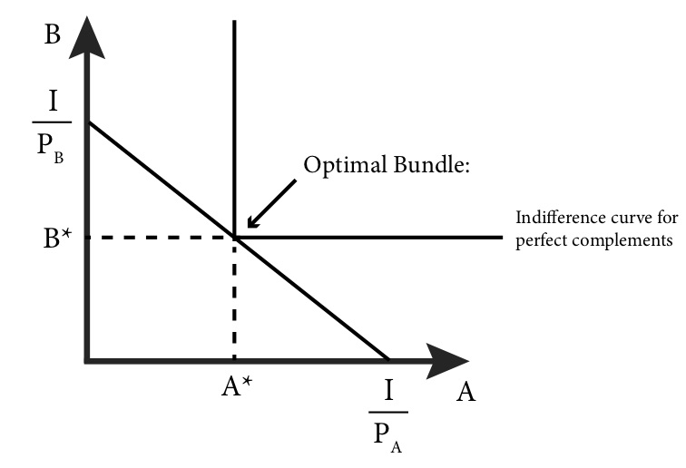
Since perfect complements have indifference curves that are kinked: they have abrupt changes in slope at a single point. At this kink, the MRS is not defined because there is no slope. The solution to the consumer choice problem with perfect complement preferences is interior – you definitely need some of both good to get any utility – but at the kink so there is no MRS to equate to ERS.
The solutions to consumer choice problems with perfect complement preferences are usually corner solutions: a utility maximizing bundle that consists of only one of the two goods. In other words, a consumption bundle that is located at one corner of the budget constraint. Corner solutions are typical when preferences are perfect substitutes but can occur for many other preference types that we will not study.
Let’s see how to find the utility maximizing bundle for these two preference types starting with perfect complements.
In the case of perfect complements with strictly positive prices, the optimal bundle is always the one at the 90-degree kink in the indifference curve, as shown in Figure 4.3. We sometimes refer to the optimal bundle with the minimum combined individual units of
Figure 4.3 Solution to the consumer choice problem for perfect complements
Recall that the utility function for perfect complements looks like this:
POP UP TEXT: Parameter: a fixed value given outside the model, one that never changes. Variable: a value that can change such as prices, income, etc.
Consuming at the kink implies that
Solving for B:
Solving for A using
Again, we see that the quantity demanded of each item decreases with an increase in its price and increases with increases in income. But now we also have the interesting result that quantity demanded of one good decreases as the price of the other good increases. This makes intuitive sense because perfect complements are goods, such as hot dogs and hot dog buns, that are only consumed together.
With perfect substitutes, the optimal bundle is generally either at one corner of the budget constraint or the other. If you stop and think about it for a moment, the intuition behind this observation becomes clear. If you like Coke and Pepsi equally well and think of them as perfect substitutes for one another, you will logically buy only the one that has the lower price. If Coke costs $1 and Pepsi $1.50, and you like them equally well, why would you ever buy any Pepsi at all? There is one exception to this “all-of-one-or-the-other” rule. When Coke and Pepsi have the same prices, you can get all of one, all of the other, or any combination of both. In this case, there is not just one optimal bundle. In this module, we will concentrate on the case where there is one optimal bundle and so you, the consumer, have to purchase all of one or the other.
Consider Figure 4.4, which illustrates a generic budget line (in black) for goods A and B, and a series of indifference curves (in blue) representing preferences for the perfect substitutes of goods A and B. The slope of the indifference curves (the MRS) is always greater than the slope of the budget line (the ERS). As you can see from Figure 4.4, this means that consumers always does better when they consume more A and less B – consumers move to a higher indifference curve. Specifically, consider bundle 1 in the graph. This bundle contains both A and B. If we compare bundle 1 to the bundle in the corner of the budget constraint labeled ‘optimal bundle’, you can see that the optimal bundle is on a higher indifference curve, which means that this bundle is better. In fact this is true of any other bundle in the budget constraint – all other bundles place consumers on a lower indifference curve.
Figure 4.4: Solution to the consumer choice problem for perfect substitutes
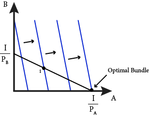
Finding this optimal bundle is relatively easy mathematically. Since we know it has to be at a corner , we just need to check the two corners of the budget constraint and see which one yields the higher utility. In general, utility functions that represent perfect complements look like this:
Note that the additive form of the utility function is the key—you can always get to the same utility by taking away some of one good and adding some of the other (even if there is none of the the other good in the bundle). Note also that the MRS is:
Since α and β are parameters, this means the slope of the indifference curve is a constant and so the indifference curves for perfect substitutes are straight lines that intersect the axes.
Solving for the optimal consumption bundle for perfect complements starts with checking the corners, which means we ask what utility the consumer gets from spending all of his or her income on just one good. So, if:
and the consumer decides to consume only A, then the total amount consumed of A is:
Similarly the total amount consumed of B if all of the income is spent on B is:
So, all that is left to do is to check whether:
or if the opposite is true or if they are equal.
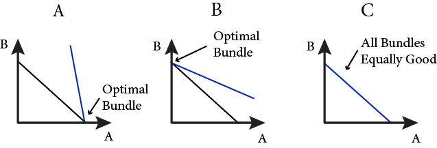
If the above is true then we know immediately that consuming only A is the optimal choice. Similarly if the opposite is true, we know consuming only B is optimal. Finally if they happen to be equal, any combination of A and B consumption along the budget line is optimal. Figure 4.5 illustrates these three possibilities.
Figure 4.5 Solutions to the consumer choice problem for perfect substitutes. Solutions (a) and (b) show the corner solutions.
SUMMARY
Review: Topics and Related Learning Outcomes
4.1 Understanding the consumer choice problem – utility maximization
LO1: Define the consumer choice problem
4.2 Solving the consumer choice problem
LO2: Solve a consumer choice problem with the typical utility function
4.3 Corner solutions and kinked indifference curves
LO3: Solve a consumer choice problem with utility function for perfect compliments and perfect substitutes.
Learn: Key Terms and Graphs
Terms
Graphs
Solution to the general consumer choice problem
Solution to the consumer choice problem for perfect substitutes
Solution to the consumer choice problem for perfect complements
Equations
Supplemental Resources
Practice Questions
YouTube Videos
These videos from the YouTube channel ‘Department of Economics’ may be helpful.
Policy Example
Policy example: The hybrid car tax credit and consumer choice
Suppose you are a policymaker considering proposals to reduce the consumption of fossil fuels and carbon emissions. With the tools from Modules 1 through 4, you can now conduct an economic analysis to analyze the likely outcome of a tax credit for electric and hybrid cars. Begin by considering the consumer choice problem prior to the introduction of the tax credit.
First, combine the indifference curve mapping from Modules 1 and 2 with the budget constraint from Module 3, as shown in Figure 1. Remember, these are simply graphical representations of the mathematical equations (equations 4.4 and 4.5).
Figure 1 Optimal Miles Driven without Car Tax Credit
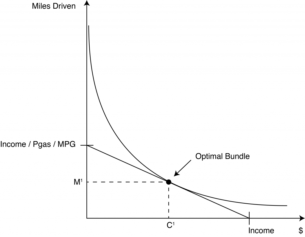
We are looking for the point on the budget line that puts the consumer on the highest indifference curve possible. This is of course the tangency point between the the indifference curve and the budget line. This tangency is characterized by the equality of the marginal rate of substitution between miles driven and other goods consumed, and the price ratio of the same two goods, the economic rate of substitution. Figure 1 shows that , given our assumption of convex indifference curves, there is a unique point that defines a number of miles driven and an amount of money for other goods consumed that make up the optimal bundle for this ‘typical’ consumer.
Mathematically, we can solve for the tangent point by remembering that it is characterized by two things:
1. The equality of the marginal rate of substitution to the price ratio.
2. The budget constraint holding with equality.
The first equation ensures that the bundle is at a point of tangency between the indifference curve and lines with the same slope as the budget line. But remember that the price ratio describes the slope, not the specific budget line, which is why we need the second equation to make sure we are on the specific line that describes the consumer’s budget.
Specifically, if the utility function that represents the ‘typical’ consumer’s preferences over miles driven (M) and all other consumption (C) is:
Then we can solve for the MRS:
As noted above, this is one condition that characterized the optimal consumption bundle, the other is the budget line:
Income = (PriceMileDriven ) x (MilesDriven) + $ for other consumption
We can solve this system of equations by the process of repeated substitution to come up with the description of the precise optimal bundle for this consumer.
Now let’s consider what happens after policymakers pass the tax credit into law. From Module 3, we know that the effect of the tax credit on the budget constraint is to make the cost of miles consumers drive less expensive, which represents a drop in the price of miles driven. This will cause the budget line to expand along the vertical axis, but it will not change the horizontal intercept. The consumer must now choice a new the optimal bundle, and we must compare the new bundle to the old one. Let’s first examine this graphically, in Figure 2.
Figure 2: Optimal Miles Consumers Drive with Car Tax Credit
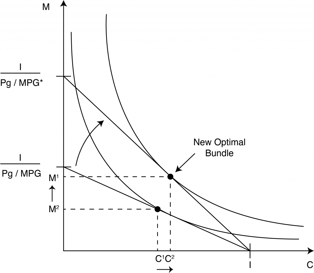
In this graph, it is clear that the new bundle represents more of both goods. The consumer will choose to consume more other goods with the extra buying power that the more fuel-efficient car affords as well as to consume more miles driven due to the lower cost of the activity. So the policy turns out to have an unintended consequence: in an effort to decrease fuel consumption, the policy actually lowers the marginal cost of driving, inducing consumers to drive more.
By making some fairly basic assumptions about typical consumer preferences and modeling the consumer choice problem, economic theory suggests that we should expect an increase in miles driven as a result. This application illustrates the power of models. By simplifying reality into a model framework, we can discover something about the world and human behavior that was not obvious.
But this is just a theory, so it is suggestive rather than definitive. It is important to note that the assumptions we made may not be completely accurate and so our prediction may be inaccurate. For example, depending on the precise indifference curve mapping we could actually see decreased miles driven after the hybrid car tax credit
We now need to test the theory by evaluating real-world data. So, what does the data suggest? Studies have shown that:
1. An increase in MPG increases how much consumers drive
2. This effect is in the rage of 10 to 30 percent, meaning that a 10 percent increase in MPG would increase how many miles consumers drive by between 1 and 3 percent.
This data does not mean that the policy is a failure. If you increase MPG by 50 percent and miles driven increase by 10 percent in response, you still have succeeded in decreasing fuel consumption substantially. The point is that you do not get the same decrease you would have expected if you didn’t understand the consumer choice problem and how consumers respond to changes in relative prices. Understanding consumer choice is important because there may be a number of different policy approaches, each with its own costs and benefits, and the goal of policymakers is to achieve the policy objective at the lowest cost.
In this case of fuel consumption, economists generally prefer that policymakers increase the gas tax, the subsidy approach and other indirect approaches like the corporate fuel economy standard known as CAFE [http://www.nhtsa.gov/cars/rules/cafe/overview.htm (inactive link as of 05/24/2021)]. The tax on fuel raises the cost of consumption and, as we have now seen, which would decrease fuel consumption. A number of studies have shown that an increase in the gas tax is a more cost-effective way to decrease gasoline usage. [http://www.cbo.gov/ftpdocs/51xx/doc5159/03-09-CAFEbrief.pdf (inactive link as of 05/24/2021)]
With our analysis of the policy based on both theory and evidence, we are now in a position to answer the original question posed at the beginning of Section 1:
Suppose that a hybrid car tax credit were wildly successful and succeeded in doubling the average fuel economy of all cars on U,S, roads . . . What do you think would happen to the fuel consumption of all U.S. motorists? Should the government expect the fuel consumption and carbon emissions of cars driven in the United States to decrease by half in response?
The answer is clearly ‘no.’ Even the most conservative estimates suggest that a 100 percent increase in average fuel efficiency will result in an increase of miles driven by 10 percent meaning that the decrease in fuel consumption and carbon emissions will fall but by less than half.
Exploring the Policy Questions
- Suppose the hybrid car tax credit were accompanied by a tax increase on gasoline. How would the analysis of the policy change? Could you make a prediction about the change in carbon emissions now?
- How would the analysis change if consumers’ preferences change and they begin to lower their gas consumption by carpooling, walking, and biking more instead of driving? How could you show this on Figure 2?
- The phenomenon of increased energy efficiency leading to increased consumption is known among economists as the rebound effect, and it is common in other practical contexts besides vehicles and driving. What other examples of rebound effect would you expect to see in the real world?
is the general term used by economists to describe the determination of the consumer’s optimal choice among competing bundles
are mathematical functions that describe the relationship between quantity demanded and prices, income and other things that affect purchase decisions
is the term used when the solution for the consumer choice problem exists within the graph's area, as opposed to on an axis
refers to a sharp bend in a line on a graph
is the term used when the solution to the consumer choice problem lies on an axis, as opposed to within the graph's interior area
are goods that consumers want to consume only in fixed proportions
is a good that is made up of a combination of individual goods. For example, a pizza is a composite good made up of dough, sauce, cheese, and other products.
is a fixed value given outside the model - one that never changes (a constant)
is a value that can change - such as prices, income, or quantity
are goods about which consumers are indifferent as to which to consume

